Multi-Objective Evolutionary Algorithm for Illiteracy Problem

International Conference on Technology and Business Management

March 23-25, 2015

Multi-Objective Evolutionary Algorithm for Illiteracy Problem Sherif Mazen Assem Tharwat Mohammed Nour El- Dien Cairo University ([email protected]) ([email protected]) ([email protected]) Shaimaa Talaat Amin Aamer Banha University ([email protected]) Multi-Criteria Decision Making MCDM has made valuable contributions to the development of various Decision Support System subspecialties. Many real-world problems have multiple competing objectives and can often be formulated as multi-objective optimization problems. Multi-objective evolutionary algorithms (MOEAs) have proven very effective in obtaining a set of trade-off solutions for such problems.This research will discuss the Multi-objective Optimization problem related to illiteracy problem. If any nation aimed at the advancement of its future should be trying to fight against many problems including illiteracy. This paper will describe the illiteracy problem in a certain city in Egypt, and study the problem to build literate classrooms at different suitable locations according to some criteria and constraints. The problem under consideration will be formulated as a multi-objective optimization model and will be solved by using one of the MOEAs that called Strength Pareto Evolutionary Algorithm (SPEA). Keywords: Mathematical Model; Multi-objective Optimization Models; Strength Pareto Evolutionary Algorithm; Genetic Algorithm; Multi-Criteria Decision Making

1. Introduction Multi-objective optimization (MO) is a hot research topic because many real life optimization problems consist of conflicting objectives. So a MO problem (or MOP) can be formulated as obtaining the best possible solutions that satisfy these objectives under different tradeoff situations. A family of solutions in the feasible solution space forms a Pareto-optimal front, which describes the tradeoff among several contradictory objectives of an MOP. The locations’ decision making problems have spatial (geographical) information, and it represent a major part of operations research and management science. Facility location is a branch of operations research related to locating or positioning a new facility among several existing facilities in order to optimize the given objective function, either profit, cost, coverage distance, or market shares [6]. This paper will discuss the illiteracy problem (IP) for a certain city in one of the Egyptian provenance. Illiteracy is one of the important problems that must be addressed and efforts should be put to help people facing it by offering the mechanisms to eliminate or decrease the illiterates. IP will be aimed to build classes for illiterate people to learn them the basics concepts for read and write. There are many attracting factors that encourage residents to go to these classes, like classes’ locations (must be close to the homes of residents), transportation cost (must be reasonable and suitable). One of the critical factors affecting the construction processes of those classes is the building cost (must be minimized), and the running cost of the class (teaching cost – it could be reduced by selecting teachers from the local residents as much as possible). Also the transportation time for the residents to the location of the class could be considered one of the factors that should be included to the problem constraints. From the budget point of view, the number of actual classes should not exceed the planned number of classes, in other words the actual building cost should not exceed the planned cost and the total actual cost should not exceed the total planned cost, and also the capacity of classes should exceed the target number of illiterates. Restrictions like the budget that covers the teachers’ compensations, and the material costs should not exceed the planned one for those purposes, and the total transportation time and distance also should be within (less than or equal) the planned total values [10]. The main target of the IP proposed model is determining of the locations for the required classes and assigning the number of students in each class. In this article it is assumed that the enrolled illiterates in each class will be at most 20 students, this will be presented as an integer variable in the suggested model. While the decision variable that indicates the effectiveness of the final decision for building a class in a certain region will appear as a binary variable in our model (1 if the decision is YES and 0 if the decision is NO) In [10] a mathematical model was introduced and the problem under investigation was formulated as a multi-objective optimization problem with 5 different objectives and more than 30 constrains covering all the above mentioned restrictions. In this paper, an optimization approach is introduced to solve the IP and to choose the best locations [9].

546


March 23-25, 2015

Recently several evolutionary algorithms (EAs) have been proposed to solve MOPs. The strength Pareto evolutionary algorithm (SPEA) [3] and the revised non-dominated sorting genetic algorithm (NSGA-II) [6] (Deb et al., 2002) are two examples for those types of algorithms [1]. In this work the authors suggest the Strength Pareto Evolutionary Algorithm (SPEA) to solve and to determine the best locations for the classes to learn the illiteracy students according to the above factors and constraints as results of applying the SPEA on the described MOP. The layout of this article is as follows: Section II introduces the illiteracy problem definition, section III describes the SPEA, Section IV discusses the IP as a MOOP, in section V the solution of the IP using the SPEA will be introduced, sections VI & VII discuses the crossover and mutation operators, finally the paper concludes with some future work will be presented in section VIII.

2. Illiteracy Problem Definition The main interest of MOP in practice is to sort out of obviously dominated solutions, rather than determine the single best design. The result is the identification of the small subset of feasible solutions (the set of non-dominated solutions) that are worthy of further consideration [5]. The problem under consideration is a city that includes a lot of centers, each center includes a lot of local units, and each local unit contains a lot of villages [9]. The ultimate goal of the problem in hand is to select the best sites to establish literacy classes for illiteracy persons and to determine the number of registered students in each class. To utilize the obtained solution of the problem it must keep in mind the three transportation restrictions (cost, time, and distance) on the following three different levels village level, local unit level, and the center level. These types of restrictions will affect directly in determining the location of the creating facility [10]. In other words, the total cost for all allocated classes in each village, local unit, and center should not exceed the available budget for establishing new classes in a village, local unit, and center, respectively. The total cost of all allocated literacy classes includes Building cost (establishing the class at a location with blackboard and chalks) and Running cost (overheads and teacher costs). The building and running cost must not exceed the available building and running budget in a village level, local unit level, and a center level. The transportation factors to reach the allocated class are important restrictions for the residents; it is includes transportation cost, transportation time, and transportation distance [10], in order to motivate the illiterate persons to attend literacy classes; we should keep in consideration the rationalization of these three types of restrictions. Starting with the restrictions belongs to the village, the number of allocated classrooms in each village and the registered students of all allocated classrooms mustn’t exceed the maximum number of allocated classes in a village and the maximum number of all illiterate persons in a village respectively [10]. Also the transportation cost of all illiterate registered students in all allocated classes should not exceed the transportation cost allocated for the village. However the total transportation time for all the students to reach the all allocated classrooms should not exceed the transportation time allocated for the village. Finally the transportation distance of all registered students in all allocated classes should not exceed the planned transportation distance for the village. There are some restrictions belong to the whole city with all centers, these restrictions contain sup-restrictions (lower level constraints) for the allocated classes in all centers and restrictions for the illiterate students in all classrooms in all centers, and it must not exceed the maximum number of classes could be allocated in the whole city. The total cost for establishing classrooms in all villages in all local units in all centers for the whole city mustn't exceed the available budget for establishing classes in the proposed governorate under consideration. The transportation cost of all illiterate persons in all allocated classes in all villages in all local units in all centers for the whole city mustn't exceed the transportation cost allocated for the whole governorate. The transportation time of all illiterate persons in all allocated classrooms in all villages in all local units in all centers for the whole city mustn't exceed the transportation time allocated for the whole governorate. The transportation distance of all illiterate persons in all allocated classrooms in all villages in all local units in all centers for the whole city mustn't exceed the available transportation distance for the whole governorate [10]. There is a critical assumption of the location illiteracy problem concerning the maximum number of students (20 students) per each class. One of the main targets to the IP is the maximization of the number of allocated classes in the best locations according to all previously discussed circumstances for the whole city [10].

3. Strength Pareto Evolutionary Algorithms (SPEA) Genetic algorithms (GAs) have been extensively used as search and optimization tools in various problem domains [5] GA allows desirable features to be passed from parents to children and discourage undesirable ones. For this purpose the two following strategies are generally useful: Crossover (methods that generate the child chromosomes by the recombination of at least two genes in parental chromosomes), and Mutation (techniques that produce a “new” solution by changing genes in the “old” chromosome). There are many approaches could be used for the IP. In this paper concentration will be directed to solve the mathematical model by the using the Strength Pareto Evolutionary Algorithm (SPEA) [3].

547


March 23-25, 2015

Zitzler and Thiele (1998a) proposed an evolutionary algorithm (SPEA) that introduces elitism by explicitly maintaining an external population (ExtPop), it stores a fixed number of the non-dominated solutions that are found until the beginning of a simulation. At every generation, newly found non-dominated solutions are compared with the existing external population at every generation, and the resulting non-dominated solutions are saved. The SPEA doesn’t just keeping the elites but using it to contribute in the genetic operations along with the current population in the hope of affecting the population to trend towards good regions in the search space [5]. Assume that the kth population is created randomly by popk of size M, and the external population will be ExtPopk with a maximum capacity MaxM , at every generation k, newly found best non-dominated solutions are kept and the dominated solutions are deleted. These non-dominated solutions are copied for the external population, in other words the ExtPopk contains old and new elites, the comparison will be occur between these elites and the resulting non-dominated solutions will be preserved in ExtPopk and all dominated solutions are deleted. By repeating the process over many generations consequently an exacerbated problem will occur by overcrowding of the external population with non-dominated solutions. In order to restrict the population to over-grow, the capacity of the ExtPop is bounded by a limit MaxM, that is means that when the size of the ExtPop is less than MaxM, all elites will preserved in the population, however, when the size exceeds MaxM, not all elites can be accommodated in the ExtPop [5]. This will be a problem because Elites which are exceeding of MaxM will not be kept. The researchers suggested a clustering method to solve this problem [5]. Once the new elites are preserved for the next generation, the algorithm then turns to the current population and uses genetic operators to find a new population. The main idea is the following: in the first step each solution in the population is assigned fitness. In addition to the assigning of fitness to the current population members, fitness is also assigned to ExtPop members. In fact, the SPEA assigns fitness strength (S) to each member (t) of the ExtPop [5]. The strength (St) is proportional to the number (numt.) of the current population members that is an external solution t dominates: St = numt (1)  M 1

The above equation assigns more strength to elite which dominates more solutions, in the current population. Division by (M + 1) ensures that the maximum value of the S of any ExtPop member is a proper fraction. A non-dominated solution dominating a fewer solutions has a smaller (or better) fitness [5].Thereafter, the fitness of a current population member b is assigned as one more than the sum of the strength values of all external population members which weakly dominate b: Fitb= 1 

S

(2)

t textpopk ,t b

The above method of fitness assignment suggests that a solution with a smaller fitness is better. Adding one in the above formula makes the fitness of any current population member Popk greater than the fitness of any external population member ExtPopk [5]. SPEA population members dominated by many external members get large fitness values, with these fitness values, a binary tournament [8] procedure is applied on the combined population (ExtPopk U Popk) to choose solutions with smaller fitness values. Thus, it is likely that external elites will be emphasized during this tournament procedure. As usua1, crossover and mutation operators are applied to the mating pool and a new population Popk+1 of size M is created [5]. For this work, the Strength Pareto Approach for multi-objective optimization has been used [3].

4. Iliteracy Problem as MOOP The general formulation of the IP under investigations consists of five different and conflicting objectives functions, the following will explain it: the 1st objective indicates the maximization of the allocated classes number, the 2nd objective represents the minimization of the allocated classes cost, the 3ed objective will minimize the total transportation cost, while the 4th objective reflects the minimization of the total transportation time, finally the 5 th objective minimizes the total transportation distance. The mathematical presentation of the above five objective functions for the multi-objective illiteracy problem (MOIP) are given as follows [3]: n

n(i )

m ( j ( i ))

   i 1

j ( i ) 1

n

n(i )

  i 1

j ( i ) 1

n

n (i )

n

(3)

X ij(i)k(j(i))c(k(j(i)))

m ( j ( i ))

l(k(j(i)))





Tcost ij(i)k(j(i))c(k(j(i))) X

(4)

ij(i)k(j(i))c(k(j(i)))

k ( j ( i )) 1 c(k(j(i))) 0

m ( j ( i ))

l(k(j(i)))



(5)

STCOSTij(i)k(j(i))c(k(j(i)))NR ij(i)k(j(i))c(k(j(i)))X ij(i)k(j(i))c(k(j(i)))

j (i )1 k ( j ( i )) 1 c(k(j(i))) 0

n (i )

m ( j ( i ))

   i 1



k ( j ( i ))1 c(k(j(i)))  0

   i 1

l(k(j(i)))

j (i ) 1

l(k(j(i)))



(6)

STTIME ij(i)k(j(i))c(k(j(i)))NR ij(i)k(j(i))c(k(j(i))) X ij(i)k(j(i))c(k(j(i)))

k ( j ( i )) 1 c(k(j(i)))0

548

International Conference on Technology and Business Management n

n(i )

m ( j ( i ))

l(k(j(i)))

    i 1

j ( i ) 1

March 23-25, 2015

(7)

STDISTij(i)k(j(i))c(k(j(i)))NR ij(i)k(j(i))c(k(j(i))) X ij(i)k(j(i))c(k(j(i)))

k ( j ( i )) 1 c(k(j(i))) 0

Where i: represents the ith center , i = 1,2,…..,n j(i): represents the jth local unit in the ith center, j(i) = 1,2,…,n(i) K(j(i)): represents the kth village in the jth local unit in the ith center, k(j(i)) =1,2,…,m(j(i)) C(k(j(i))): represents the cth class in the kth village in the jth local unit in the ith center , c(k(j(i))) = 1,2,…, l(k(j(i))) X ij(i)k(j(i))c(k(j(i))): it is one of the model decision variables, it takes the value 1 if the lth class located in kth village in jth local unit in the ith center, and takes o otherwise th NRij(i)k(j(i))c(k(j(i))): it is another one of the model decision variables, it represents the number of registered students in the c th th th class in the k village in the j local unit in the i center. Tcost ij(i)k(j(i))c(k(j(i))): represents the total cost of the cth class in the kth village in the jth local unit in the ith center Total cost of each class equals the sum of the construction (building) cost of the class and the running (teaching) cost of the class. STCOSTij(i)k(j(i))c(k(j(i))): represents the transportation cost to the cth class in the kth village in the jth local unit in the ith center STTIMEij(i)k(j(i))c(k(j(i))): represents the transportation time to the cth class in the kth village in the jth local unit in the ith center STDISTij(i)k(j(i))c(k(j(i))): represents the transportation distance to the cth class in the kth village in the jth local unit in the ith center The second objective calculates the grand total cost by adding the total costs for only the effective classes. While the third one calculates the grand total transportation costs, by adding the total transportation costs (depend on the number of registered students in each class) for only the effective classes. The 3ed and the 4th objectives act like the second with respect to the time and distance. The complete description of the IP set of constraints based on the above discussion in section II is given in the Appendix. Four different sets of constraints are mentioned: the first set related to the total number of classes covering the three levels, village, local unit, and center and also the aggregate provenance level, the second set of constraints related to the number of illiteracy inhabitants covering the three levels, the third and the fourth sets of constraints related to the facility costs, and the transportation costs respectively and covering the three spatial levels beside the provenance aggregation level.

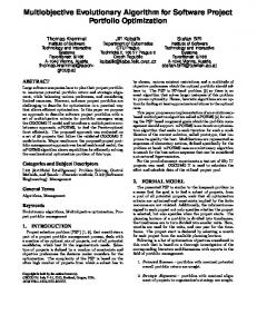
5. Generalized SPEA: MOOP Application (1) Chromosome Representation The chromosome structure for the problem at hand contains two parts as in Fig1 [10], the first one is the binary part for X (a binary decision variable represents the class location status) and the second one is a the real part for NR (an integer decision variable represents the number of registered students) The proposed problem requires a chromosome to encode the decision variables related to the research problem, the length of the required chromosome is twice the suggested number of locations that the user will choose them in our application. Assume that the chromosome length (Chlen), and assume that the suggested number of locations is 6, so Chlen = 12.

Figure 1 Chromosome Structure

(2) Evaluation Phase A Genetic Algorithm begins its search with a set of solutions randomly. Once a random population of solutions (a random set of binary/real strings is created, each is evaluated in the context of the underlying problem and fitness is assigned to each solution t. The evaluation of a solution means calculating the objective function value and constraint violations as in table I. Thereafter, a metric must be defined by using the objective function value and constraint violations to assign a relative merit to the solution (fitness) [4]. So the substitution is done by each solution of random population to calculate the values of the five objective functions and the 296 constraints violations. The constraints divide the search space into two divisions – feasible and infeasible regions. The popular approach to handle the optimization problems with constraints is the Penalty function approach [4].

549


March 23-25, 2015

Table 1 Fitness Assigment for Objective Function Solution func1 func2 func3 func4 func5 1 0 0 0 0 0 2 -3 8000 2514 2514 20880.8 3 -4 18000 1410 1410 57956.3 4 -5 23400 379 379 68239.7 5 -2 13400 186 186 46593.6

(3) Penalty function Approach Penalty function approach is a popular constraint handling strategy. The minimization of all objective functions is assumed in the described model; however, the duality principle will be applied to handle a maximization function by converting the maximization function to minimization function. For each solution y(t), the constraint violation for each constraint is calculated as follows [4]: convj (y(t))= | h j ( y (t) ) |, if

(8)

h j ( y (t) )  0

  0 , otherwise

Thereafter, all constraint violations are added together to get the overall constraint violation: sconv(y(t))=

J

(t)

conv (y j

(9)

)

j1

Multiply the constraint violation by the penalty parameter Rm and the product is added to each of the objective function values [4]: FUNCm(y(t) ) = funcm (y(t)) + R m (sconv(y(t)))

(10)

It is clear that the function FUNCm takes into account the constraint violations, and for a feasible solution, the corresponding sconv term is zero and hence FUNCm becomes equal to the original objective function funcm. However, for an infeasible solution the value of FUNCm will be greater than funcm, thereby adding a penalty belongs to the total constraint violation i.e. sconv term will be positive. The penalty parameter Rm is used to make the two terms on the right side of the above equation to have the same order of magnitude [4].Once the penalized function is formed, any of the unconstrained multi-objective optimization methods can be used with FUNCm as in table II. Table 2 Penaliz Ed Function Values of all Five Solution F (Pt) Sconv FUNC1 FUNC2 FUNC3 FUNC4 FUNC5 0 0 0 0 0 0 7154 3576997 49299060 1433314 1647934 12898080 1750 874996 12075500 351410 403910 3207956 0 -5 23400 379 379 68239 0 -2 13400 186 186 46593

(4) SPEA for Illiteracy Problem Assume that Chlen =6, Population size (M) = 5, and ExtPop size (MaxM) =3. SPEA Initialized by, ExtPopk =  (assummution). In the first generation k, ExtPopk = FUNC (Popk) In the first step of SPEA Algorithm, the best non-dominated set FUNC (Popk) of Popk will be obtained, copy these solutions to ExtPopk . In the second step for SPEA Algorithm, the ExtPopk includes the (old elites) previous non-dominated solutions, if exists, and the new elites for this generation, the best non-dominated solutions FUNC(Popk) will be found as in table III after the comparison with elites in ExtPopk , and delete all the dominated solutions, or perform ExtPopk = FUNC(ExtPopk ). Table 3 External Population with their Objective Functions Values Solution FUNC1 FUNC2 FUNC3 FUNC4 FUNC5 1 0 0 0 0 0 4 -5 23400 379 379 68239 5 -2 13400 186 186 46593

In the third step for SPEA Algorithm, If |ExtPopk| > MaxM, use a clustering technique to reduce the size to MaxM. Otherwise, keep ExtPopk unchanged. Hence the resulting population is the external population ExtPopk+1 of the next generation.

550


March 23-25, 2015

In our case study, if |ExtPopk | < MaxM, so keep ExtPopk unchanged. For the first generation, the ExtPopk will be empty and retain non-dominated solutions. The resulting population is the external population ExtPopk+1 in table III for the next generation and will be compared with the new elites in K+1 generation. In the fourth step of SPEA algorithm, assign fitness to each elite solution by using equation 1. Then, assign fitness to each population member b  Popk by using the equation 2. SPEA assigns a fitness St to each member t of the external population as in table IV. Table 4 New Fitness Assignment for Objective Values (Strength For All Solutions) Solution Strength for all solution 1 0.333333 2 2 3 2 4 0.333333 5 0.333333

In our study, If |ExtPopk | > MaxM, use a clustering technique to reduce the size to 3. It is needed to see if the external population has 5 solutions are greater than the MaxM. The clustering technique will be applied, each solution in ExtPopk is considered to reside in a separate cluster. Thus, initially there are M clusters. Thereafter, the cluster -distances between all pairs of clusters are calculated. In general, the distance dist12 between two-clusters Clust1 and Clust2 is defined as the average Euclidean distance of all pairs of solutions (t Clust1 and b  Clust2), or mathematically [5]: 1 dist12 = (11) dist(t , b) ss | Clust1 || Clust 2 |



tclust1, bclust 2

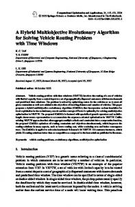
In our study, a binary tournament selection [8] will be applied with these fitness values (in a minimization sense), a crossover and a mutation operator (see the next sections) to create the new population ExtPopk+1 of size M from the combined population (ExtPopk  Popk) of size (MaxM+ M) [4]. (5) CROSSOVER Operators The crossover process creates two new strings (called offspring). Since a single cross site is chosen in this work, the couponing crossover operator is called the single-point crossover operator [7]. In a single-point crossover operator, the crossover is performed by randomly choosing a crossing site along the string in the interval [0,(Chlen/2)] and by exchanging all bits on the right side of the crossing site [5]. In the proposed problem, the single-point crossover operator will be applied for the binary part in the chromosome structure (X). While the crossover operator for the real Part of the chromosome (NR) could be any operator that combines the genetic material of two parents, call it the recombination operator. Let a = (a1,a2,…….,am) and b = (b1,b2,……..,bm) be the parent strings [7]. Then the offspring c = (c1,c2,……..,cm) is computed by ci = ai +  i (bi - ai) such that i=1,2,……m,  i is chosen uniform randomly in the interval [-0.25,1.25], Fig.2 applied the crossover operator for the problem under consideration.

Figure 2 The Crossover Operator for the Real Part for Illteracy Problem

(6) Mutation Operators The bit-Flipping mutation procedure will be applied for the binary part for a chromosome structure as in Fig 3. The bitFlipping mutation operator changes from 1 to 0, and vice versa, with a mutation probability of mutp (mutation rate = 0.1) [4,5]. The bit-Flipping mutation procedure requires choosing a bit, then creating a random number belongs to [0,1] for every time the crossover operator emerged offspring. So if the random number is less than mutp, then changes the chosen bit from 1 to 0, and vice versa. Otherwise, don’t change the chosen bit [4,5]. The mutation procedure will be applied in the mutation step for the SPEA approach.

Figure 3 Fig.Bit-Flipping Mutation

551


March 23-25, 2015

The Gaussian mutation procedure will be applied for the real part in a chromosome structure; this algorithm will be applied for the problem under consideration [4]. The Gaussian mutation will be operated to determine the optimized locations for building classes for illiteracy students in the city. Note that before running the optimization method, some input parameters should be to determine such that, the number of solutions (locations that can be used to build classes from the chosen locations by user), the number of solutions which make the clustering procedure start in SPOPEV algorithm discussed before.

6. Conclusions and Future Work This paper discussed the illiteracy problem at a city and searched for the factors and conditions that affected for the problem. Geographically the city contains three levels of divisions, center, local unit, and village. Each city contains a number of centers, each center contains number of local units and each local unit contains number of villages. After searching around the proposed problem, it was found that the problem will be represented as the multi-objective model. MOP contains some objectives and restrictions belong to the circumstances and conditions of the city. The important target for this research is to establish literate classes in some definite locations suitable for illiterate persons in their city and suitable for their monthly income. From the statistical and social points of view, the income of the people in the city significantly affect for some factors that affected the multi-objective model like transportation cost factor for literate classes. There are a number of popular multi-objective decision making approaches are applied to solve the multi-objective decision making problems. Some Multi-Objective problems were solved by classical methods or evolutionary methods. There exist a lot of evolutionary algorithms that are applied for the multi-objective optimization problems such as anticolony optimization, simulated annealing evolution, DNA computing, Genetic algorithms, and Swarm optimization. One of the Genetic algorithms was applied for this research, called the Strength Pareto Algorithm, and it was applied for problems related to the spatially features to create some decisions. Geographic Information Systems (GIS) are mostly used in regional planning for visualizing spatial data sets. However, GIS remain the external artifacts to the decision-making approaches. So one can say that in-spite improving the analytic sophistications GIS software, but still providing limited outputs (maps, tables, etc.) than as a tool to support. To improve the usefulness of GIS as a decision support tool, the multi-objective decision making concept will be applied on the problems related to spatially feature. There are a number of popular multi-objective decision making techniques can be used to solve the problems related to spatially feature. It is suggested to integrate between the multi-objective decision making technique and GIS.

7. References 1.

C.H.Lin,and P.L.Lin," A New Non-dominated Sorting Genetic Algorithm for Multi-Objective Optimization",Department of Information Management, Chung Yuan Christian University,Taiwan, 2010. 2. H. Yassami, A. Darabi, and S. Rafiei," Power system stabilizer design using Strength Pareto multi-objective optimization approach ", Department of Electrical Engineering, Politecnico Di Torino, Torino, Italy,2010. 3. H. Sato, H. Aguirre, and K. Tanaka," Variable space diversity, crossover and mutation in MOEA solving many-objective knapsack problems",Ann Math Artif Intell (2013) 68:197–224. 4. John Wiley, Multi-Objective Optimization Using Evolutionary Algorithms, Indian Institute Of Technology, Department Of Mechanical Engineering, ISBN 0-471-87339-X, PP. 1-2, New York, 2001. 5. K. Deb, A. Pratap, S. Agarwal, and T. Meyarivan," A fast and elitist multiobjective genetic algorithm: NSGA-II", IEEE Transactions on Evolutionary Computation , VOL. 6, NO. 2, 2002. 6. M. Braun, P. Shukla, and H. Schmeck," Preference Ranking Schemes in Multi-Objective Evolutionary Algorithms",Institute AIFB, Karlsruhe Institute of Technology, Germany,2011 7. N. Razali, and J. Geraghty,"Genetic Algorithm Performance With Different Selection Strategies in Solving TSP", Proceedings of the World Congress on Engineering, Vol II London, 2011. 8. R. Farahani, M. SteadieSeifi, and N. Asgari, "Multiple criteria facility location problems: A survey", Centre for Maritime Studies, National University of Singapore, Singapore, Department of Industrial Engineering, Amirkabir University of Technology, Tehran, Iran, 2010. 9. S. Talaat," hypermodel for GIS and decision support system ", Master (Msc) Thesis, department of information system, faculty of Computers &Information Systems, Cairo University, Giza, Egypt,2008 10. S. Mazen, A. Tharwat, M. Nour El-Dean, and S. T. Amin," Mathematical Optimization Model For The Illiteracy Problem", The 6th International Conference on Informatics and Systems, Faculty of Computers & Information, Cairo University, 2008. 11. S. Potti, and C. Chinnasamy," Strength Pareto Evolutionary Algorithm based Multi-Objective Optimization for Shortest Path Routing Problem in Computer Networks ", Journal of Computer Science 7 (1): 17-26, 2011. Appendix The proposed mathematical model for the problem under investigation has the following sets of constraints: Constraints Related the Number of Classes (NOC)

552


March 23-25, 2015

1. Cij(i)k(j(i)) l(k(j(i))) Xij(i)k(j(i))c(k(j(i)))  MNC ij(i)k(j(i))  Cij(i)k(j(i)) 1

2

Cij(i)k(j( i))  l(k(j(i)))

m( j ( i ))





k ( j (i )) 1

Cij(i)k(j( i)) 1

3

n(i)

m( j ( i ))





n

4.

Cij(i)k(j( i)) l(k(j(i)))

Cij(i)k(j(i)) 1 Cij(i)k(j( i))  l(k(j(i)))

m( j ( i ))

n(i)

  i 1

Xij(i)k(j(i))c(k(j(i)))  MNC i



k ( j (i ))1

j ( i ) 1

Xij(i)k(j(i))c(k(j(i)))  MNC ij(i)

j ( i ) 1





k ( j (i ))1

Cij(i)k(j(i)) 1

Xij(i)k(j(i))c(k(j(i)))  MNC

Where: MNC ij(i)k(j(i)): represents the maximum NOC could be located in the kth village in the jth local unit in the ith center MNC ij(i) : represents the maximum NOC could be located in the jth local unit in the ith center MNC i : represents the maximum NOC could be located in the ith center MNC: represents the maximum NOC could be located in the Governorate 5. 0  NR ij(i)k(j(i))c(k(j(i)))  20 Constraints Related the Number of Illiteracy Inhabitants (NII) 6. Cij(i)k(j(i)) l(k(j(i))) NR ij(i)k(j(i))c(k(j(i))) X ij(i)k(j(i))c(k(j(i)))  ITv ij(i)k(j(i))



Cij(i)k(j(i)) 1 m( j ( i )) Cij(i)k(j( i)) l(k(j(i)))

7.





k ( j (i ))1

8.


m( j ( i ))

n(i)

 k( j (i ))1 n

m( j ( i ))

n(i)

  i 1

j ( i ) 1

NR ij(i)k(j(i))c(k(j(i))) X ij(i)k(j(i))c(k(j(i)))  ITc i



Cij(i)k(j(i)) 1

j ( i ) 1

9.

NR ij(i)k(j(i))c(k(j(i))) Xij(i)k(j(i))c(k(j(i)))  ITl ij(i)

Cij(i)k(j(i)) 1

Cij(i)k(j(i)) l(k(j(i)))





k ( j (i ))1

Cij(i)k(j(i)) 1

NR ij(i)k(j(i))c(k(j(i))) Xij(i)k(j(i))c(k(j(i)))  IGT

Where: ITvij(i)k(j(i)): represents the NII in the kth village in the jth local unit in the ith center ITlij(i): represents the NII in the jth local unit in the ith center ITci : represents the NII in the ith center IGT: represents NII in the Governorate Constraints Related the Facility Costs Cij(i)k(j(i)) l(k(j(i)))

10.



Tccostij(i)k(j(i))c(k(j(i))) Xij(i)k(j(i))c(k(j(i)))



TVcost ij(i)k(j(i))

Cij(i)k(j(i)) 1

11.

Cij(i)k(j(i)) l(k(j(i)))



Bccostij(i)k(j(i))c(k(j(i))) Xij(i)k(j(i))c(k(j(i)))



BVcost ij(i)k(j(i))

Rccostij(i)k(j(i))c(k(j(i))) Xij(i)k(j(i))c(k(j(i)))



RVcost ij(i)k(j(i))

Cij(i)k(j(i)) 1


12.



Cij(i)k(j(i)) 1 m( j ( i )) Cij(i)k(j(i)) l(k(j(i)))

13.

 



k ( j (i ))1

16.





k ( j (i ))1

Cij(i)k(j(i)) 1

n(i)

 j ( i ) 1

17.

n (i )



n (i )

j ( i ) 1

19. 20.

n

21.

m( j ( i )) Cij(i)k(j( i)) l(k(j(i)))



m( j ( i )) Cij(i)k(j( i)) l(k(j(i)))



k ( j (i ))1 n (i )





BCcost i

Rccostij(i)k(j(i))c(k(j(i))) Xij(i)k(j(i))c(k(j(i)))



RCcost i

m( j ( i )) Cij(i)k(j( i))  l(k(j(i)))

n

n(i)



j ( i ) 1 k ( j (i ))1

j ( i ) 1 k ( j (i ))1



TTC






BTG

Cij(i)k(j(i)) 1

m( j ( i )) Cij(i)k(j( i)) l(k(j(i)))

  


Cij(i)k(j(i)) 1

m( j ( i )) Cij(i)k(j( i)) l(k(j(i)))

   n(i)


Cij(i)k(j(i)) 1

j ( i ) 1 k ( j (i ))1

n

ccostij(i)k(j(i))c(k(j(i))) Xij(i)k(j(i))c(k(j(i)))  TCcosti

Cij(i)k(j(i)) 1

i 1

i 1

 RLcost ij(i)

Cij(i)k(j(i)) 1

   i 1

Rccostij(i)k(j(i))c(k(j(i))) X ij(i)k(j(i))c(k(j(i)))



k ( j (i ))1

 k( j (i ))1



 BLcost ij(i)

m( j ( i )) Cij(i)k(j(i)) l(k(j(i)))

j ( i ) 1

18

Bccostij(i)k(j(i))c(k(j(i))) X ij(i)k(j(i))c(k(j(i)))

Cij(i)k(j(i)) 1

m( j ( i )) Cij(i)k(j(i)) l(k(j(i)))

15.

 TLcost ij(i)

Cij(i)k(j(i)) 1

m( j ( i )) Cij(i)k(j(i)) l(k(j(i)))

14.




k ( j (i ))1



Rccost ij(i)k(j(i))c(k(j(i))) Xij(i)k(j(i))c(k(j(i)))



RTG

Cij(i)k(j(i)) 1

BCcostij(i)k(j(i))c(k(j(i))): represents the building cost of the cth class in the kth village in the jth local unit in the ith center BVcost ij(i)k(j(i)):: represents the available building costs of the located classes in the kth village in the jth local unit in the ith center

553


March 23-25, 2015

BLcost ij(i): represents the available building costs of the located classes in the jth local unit in the ith center BTG: represents the available building cost of the located classes in the Governorate RCcostij(i)k(j(i))c(k(j(i))): represents the running cost of the cth class in the kth village in the jth local unit in the ith center RVcost ij(i)k(j(i)): represents the available running costs of the located classes in the kth village in the jth local unit in the ith center RLcost ij(i): represents the available running costs of the located classes in the jth local unit in the ith center RTG: represents the available running cost of the located classes in the Governorate TCcostij(i)k(j(i))c(k(j(i))): represents the Total cost of the cth class in the kth village in the jth local unit in the ith center TVcost ij(i)k(j(i)): represents the available total costs of the located classes in the kth village in the jth local unit in the ith center TLcost ij(i): represents the available total costs of the located classes in the jth local unit in the ith center TTC: represents the available total costs of the located classes in the Governorate Constraints Related the Transportation Costs 22. Cij(i)k(j(i)) l(k(j(i))) STCOSTij(i)k(j(i))c(k(j(i))) NRij(i)k(j(i))c(k(j(i)))



Cij(i)k(j(i)) 1

m( j ( i )) Cij(i)k(j( i)) l(k(j(i)))

23.





k ( j (i ))1

24.

Cij(i)k(j(i)) 1

m( j ( i )) Cij(i)k(j( i)) l(k(j(i)))

n(i)

 



j ( i ) 1 k ( j (i ))1

25.

Xij(i)k(j(i))c(k(j(i)))  MTCOSTVij(i)k(j(i)) STCOSTij(i)k(j(i))c(k(j(i)))NR ij(i)k(j(i))c(k(j(i)))

n

Cij(i)k(j(i)) 1

m( j ( i )) Cij(i)k(j( i))  l(k(j(i)))

n (i )

   i 1

Xij(i)k(j(i))c(k(j(i)))  MTCOSTLij(i) STCOSTij(i)k(j(i))c(k(j(i))) NR ij(i)k(j(i))c(k(j(i)))



j ( i ) 1 k ( j (i ))1

Xij(i)k(j(i))c(k(j(i)))  MTCOSTCi STCOSTij(i)k(j(i))c(k(j(i)))NR ij(i)k(j(i))c(k(j(i)))

Cij(i)k(j(i)) 1

Xij(i)k(j(i))c(k(j(i)))  MTCOST 26. Cij(i)k(j(i)) l(k(j(i))) STTIMEij(i)k(j(i))c(k(j(i))) NR ij(i)k(j(i))c(k(j(i)))



Cij(i)k(j(i)) 1





k ( j (i ))1

28.

Cij(i)k(j(i)) 1

m( j ( i )) Cij(i)k(j( i)) l(k(j(i)))

n(i)

 

j ( i ) 1 k ( j (i ))1

29.

n



Xij(i)k(j(i))c(k(j(i)))  MTTIMELij(i) STTIME ij(i)k(j(i))c(k(j(i))) NRij(i)k(j(i))c(k(j(i)))

Cij(i)k(j(i)) 1

m( j ( i )) Cij(i)k(j( i))  l(k(j(i)))

n (i )

   i 1

Xij(i)k(j(i))c(k(j(i))  MTTIMEVij(i)k(j(i)) STTIME ij(i)k(j(i))c(k(j(i))) NRij(i)k(j(i))c(k(j(i)))


27. m( j (i))



j ( i ) 1 k ( j (i ))1

Xij(i)k(j(i))c(k(j(i)))  MTIMECi STTIMEij(i)k(j(i))c(k(j(i)))NRij(i)k(j(i))c(k(j(i)))

Cij(i)k(j(i)) 1

Xij(i)k(j(i))c(k(j(i)))  MTTIMEG 30. Cij(i)k(j(i)) l(k(j(i))) STDISTij(i)k(j(i))c(k(j(i))) NR ij(i)k(j(i))c(k(j(i)))



Cij(i)k(j(i)) 1

Xij(i)k(j(i))c(k(j(i)))  MTDISTVij(i)k(j(i) 31. m( j (i)) Cij(i)k(j(i)) l(k(j(i))) STDISTij(i)k(j(i))c(k(j(i))) NR ij(i)k(j(i))c(k(j(i)))



k ( j (i ))1



Cij(i)k(j(i)) 1

Xij(i)k(j(i))c(k(j(i)))  MTDISTLij(i) 32. n (i ) m( j (i)) Cij(i)k(j(i)) l(k(j(i))) STDISTij(i)k(j(i))c(k(j(i)))NR ij(i)k(j(i))c(k(j(i)))

 

j ( i ) 1 k ( j (i ))1



Cij(i)k(j(i)) 1

Xij(i)k(j(i))c(k(j(i)))  MDISTCi 33. n n (i ) m( j (i)) Cij(i)k(j(i)) l(k(j(i))) STDISTij(i)k(j(i))c(k(j(i)))NR ij(i)k(j(i))c(k(j(i)))

   i 1

j ( i ) 1 k ( j (i ))1



Cij(i)k(j(i)) 1

Xij(i)k(j(i))c(k(j(i)))  MTDISTG

STCOSTij(i)k(j(i))c(k(j(i))): represents the transportation cost to reach the cth class in the kth village in the jth local unit in the ith center MTCOSTVij(i)k(j(i)): represents the Maximum transportation cost for all students to reach the allocated class in the kth village in the jth local unit in the ith center MTCOSTLij(i): represents the Maximum transportation cost for all students to reach the allocated class in the jth local unit in the ith center MTCOSTCi : represents the Maximum transportation cost for all students to reach the allocated class in the ith center MTCOSTG: represents the Maximum transportation cost for all students to reach the allocated class in the Governorate

554


March 23-25, 2015

STTIMEij(i)k(j(i))c(k(j(i))): represents the transportation time of any student to reach the cth class in the kth village in the jth local unit in the ith center MTTIMEVij(i)k(j(i)): represents the Maximum transportation time for all students to reach the allocated class in the kth village in the jth local unit in the ith center MTTIMELij(i) : represents the Maximum transportation time for all students to reach the allocated class in the jth local unit in the ith center MTTIMECi : represents the Maximum transportation time for all students to reach the allocated class in the ith center MTTIMEG: represents the Maximum transportation time for all students to reach the allocated class in Governorate STDISTij(i)k(j(i))c(k(j(i))): represents the transportation distance for each student to reach the cth class in the kth village in the jth local unit in the ith center MTDISTVij(i)k(j(i)): represents the Maximum transportation distance for all students to reach the allocated class in the kth village in the jth local unit in the ith center MTDISTLij(i): represents the Maximum transportation distance for all students to reach the allocated class in the jth local unit in the ith center MTDISTCi: represents the Maximum transportation distance for all students to reach the allocated class in the ith center MTDISTG: represents the Maximum transportation distance for all students to reach the allocated class in the Governorate

555