Multi-Objective Genetic Algorithm Optimisation of Water Distribution Systems Accounting for Sustainability Wenyan Wu, Angus R. Simpson, Holger R. Maier School of Civil, Environmental and Mining Engineering The University of Adelaide Adelaide 5005 AUSTRALIA E-mail:
[email protected] [email protected] [email protected]
Wu, W., Simpson, A.R. and Maier, H.R. (2008). “Multi-objective genetic algorithm optimization of water distribution systems accounting for sustainability”, Water Down Under Conference, Adelaide, April.
Multi-Objective Genetic Algorithm Optimisation of Water Distribution Systems Accounting for Sustainability Wenyan Wu, Angus R. Simpson, Holger R. Maier School of Civil, Environmental and Mining Engineering The University of Adelaide Adelaide 5005 AUSTRALIA E-mail:
[email protected] [email protected] [email protected] Abstract Considerable research has been carried out on the optimisation of water distribution systems (WDSs) within the last three decades. In previous research, attention has mainly focused on the minimisation of the cost of the networks. The study described in this paper extends previous research by incorporating into the optimisation an environmental sustainability criterion of minimising Greenhouse Gas (GHG) emissions. A Multi-Objective Genetic Algorithm was developed to solve this problem. The impacts of minimising GHG emissions on the results of WDS optimisation have been explored for two simple case studies: a one-pipe pumping system and one multi-pump system. In addition, results obtained from optimising WDSs accounting for both the economic and environmental sustainability objectives are compared with those obtained when only the economic objective was considered. A comparison of results indicates that the inclusion of GHG emission minimisation as one of the objectives results in significant tradeoffs betwe. en the economic objective and the environmental sustainability objective. This research will allow the consideration of sustainability criteria in the planning, design and evaluation of WDSs, and further contribute to sustainable development in urban areas.
1. INTRODUCTION Water Distribution Systems (WDSs) are essential infrastructure. Urban water consumers (domestic, commercial and industrial) rely on these systems to obtain clean water to perform basic activities (Filion, et al., 2004). Due to the high cost associated with the construction and maintenance of WDSs, there is always a need to optimise the design of WDSs in order to minimise both the cost of the design and the operating costs (Simpson, et al., 1994, Zecchin, et al., 2006). However, the impacts of WDSs on the environment usually have not been considered adequately (Ghimire & Barkdoll, 2007). Recently, a number of studies attempted to incorporate various environmental considerations, such as minimisation of energy usage (Sarbu & Borza, 1998), water quality issues (Dandy & Hewitson, 2000) and minimisation of material usage (Dandy, et al., 2006) into the optimisation of WDSs. In addition, Dandy et al. (2006) also evaluated the Greenhouse Gas (GHG) emissions of two different designs of a WDS. However, there is no current research that has incorporated GHG emissions into a multiobjective WDS optimisation. So far, only a few studies (Savic, 2002, Prasad & Park, 2004, Keedwell & Khu, 2006) have applied multi-objective algorithms to optimise the design of WDSs; however, none of these considered environmental objectives. The study described in this paper extends previous research by using a multi-objective approach to incorporate an environmental sustainability criterion into the optimisation of WDSs by consideration of minimising GHG emissions as an objective, along with economic considerations. Since sustainable development was defined by the World Commission on Environment and Development in 1987, sustainability has been widely used as a management goal in different disciplines (Hu, 1997). There are many definitions of sustainability. One of these was presented by Gilman (1992) as: “the ability of a society, ecosystem, or any such on-going system to continue functioning into the indefinite future without being forced into decline through exhaustion or overloading of key resources on which the system depends.”
MOGA Optimisation of WDSs Accounting for Sustainability
Wu
This definition can be best explained by a conceptual model, the “Sustainability Space”, which was developed by Foley and Daniell (2002). There are four dimensions: economic, environmental, social and temporal. The temporal dimension incorporates the possible changes of people’s views over time. Therefore, sustainability can be measured using sustainability indicators in these dimensions (Sahely, et al., 2005). In this study, two sustainability indicators for WDSs are used, including one economic and one environmental. The impact the temporal dimension of sustainability on the tradeoffs between the two objectives is taken into account by using Present Value Analysis (PVA). The remainder of this paper is organised as follows. The methodologies used in this study are presented in Section 2. In Section 3, the formulation of the multi-objective WDS optimisation problem is described. Thereafter, the impacts that minimising GHG emissions have on the results of WDS optimisation are explored for two simple case studies in Section 4. The results obtained from optimising WDSs accounting for both economic and sustainability objectives are compared with those obtained from existing WDS optimisation that accounts only for the economic objective. A comparison of results is also given in Section 4. Finally, conclusions are presented in Section 5.
2. METHODOLOGY
2.1. Overview This study optimises the design of WDSs accounting for both the economic and environmental aspects of sustainability. An overview of WDS optimisation and the objectives accounted for in this study are illustrated in Figure 1. This figure shows the four steps of WDS optimisation: Generation of options, Simulation, Evaluation, and Comparison and Selection. These four steps are repeated until the stopping criteria are met. Previously, Genetic Algorithms (GA) have proved to be effective for WDS optimisation (Simpson, et al., 1994). In this study, a special type of genetic algorithm, a Multi-Objective Genetic Algorithm (MOGA), is used. The details of MOGA are given in Section 2.2. As part of the optimisation process, each trial solution of the design of a WDS is passed to a simulation model for hydraulic analysis. There are many such simulation models. In this study, EPANET2 is used to solve for heads and flows in the network. These values are used in the evaluation step to compute the values of the objective functions. The methods used in the study to evaluate the two objectives include Present Value Analysis (PVA), Gamma discounting, Life Cycle Analysis (LCA), Embodied Energy Analysis (EEA) and Emission Factor Analysis (EFA). Details of these methods are given in Section 2.3 and 2.4.
2.2. Genetic Algorithms and Multi-Objective Optimisation Genetic Algorithms are global optimisation methods that belong to the class of evolutionary algorithms, which are inspired by natural phenomena (Goldberg, 1989). Genetic Algorithms use the principle of “survival of the fittest” to select more suitable solutions within a population of solutions simultaneously. A multi-objective optimisation approach is used in this study, which differs from a single-objective approach in that there exist a number of optimal solutions due to the trade-offs between conflicting objectives. An example of the tradeoffs between two conflicting objectives is shown in Figure 2. It can be seen that there are six optimal solutions, which form a Pareto-optimal front. No solution on this front is better than the others in terms of both objectives. Therefore, they are called non-dominated solutions (Deb, 2002). In order to obtain the non-dominated solutions of multiobjective optimisation problems simultaneously, a multi-objective optimisation approach, such as a multi-objective genetic algorithm, is required. Multi-objective genetic algorithms can find non-dominated solutions in one simulation run. Deb et al. (2002) suggested a non-dominated sorting based multi-objective Genetic Algorithm – NSGA-II, which overcomes disadvantages of traditional multi-objective algorithm optimisation approaches. Previously, genetic algorithms have had a disadvantage relating to the handling of constraints, as they require additional parameters in the form of penalty coefficients (Prasad & Park, 2004). In order to take
WATER DOWN UNDER 2008 Wu, Simpson, Maier
2 of 12
MOGA Optimisation of WDSs Accounting for Sustainability
Wu
account of constraints in a better way, Deb (2000) introduced an efficient constraint handling method for GAs referred to as constrained tournament selection (Deb, 2002).
WDS Optimisation Generate Options Simulation MOGA Evaluation Comparison & Selection
Two objectives Economic
Environmental Total cost
GHG emissions LCA
Capital cost
Operating & Pump replacement cost
Capital emissions EFA Energy use
PVA (Single discount rate/Gamma discounting)
Operating emissions PVA (Single discount rate/Gamma discounting)
EEA Life cost
Material use
Life GHG emissions
Figure 1 Overview and Objectives of WDS Optimisation
Objective 1 Optimal solutions Pareto-optimal front
Objective 2
Figure 2 Tradeoffs between two conflicting objectives A Multi-Objective Genetic Algorithm for water distribution system optimisation has been developed in this research based on NSGA-II and the constrained tournament selection method. Instead of using a traditional binary coding scheme, the inputs of the GA have been modified to be either integers or real numbers, which caters for the different types of decision variables encountered in WDS optimisation.
2.3. Evaluation of Total Cost The first objective in the WDS optimisation problem is to minimise the total cost of the system. It can be seen from Figure 1 that the total network costs considered in this study consist of three parts: capital costs, operating costs and pump replacement costs. The capital cost is the initial investment, which mainly comes from the purchase and installation of network components. The capital costs
WATER DOWN UNDER 2008 Wu, Simpson, Maier
3 of 12
MOGA Optimisation of WDSs Accounting for Sustainability
Wu
occur at the beginning of a project. In this study, operating costs are mainly due to electricity consumption related to system operation. Both operating costs and pump replacement costs occur during the whole life of the network. Consequently, the evaluation of these two costs requires Present Value Analysis (PVA). Present Value Analysis Present value analysis is a fundamental activity in economics, as it addresses the problem of the time value of money (Bagamery, 1991). With an appropriate discount rate, present value analysis translates values from the future to the present, enabling effects occurring at different times to be compared (Kaen, 1995). The Present Value (PV) of a future payment can be calculated using the following equation:
PVt =
C (1 + i )t
(1)
t is the number of periods; i is the discount rate. PVt is the Present Value of a future payment at the end of the t th period. Similarly, the
where, C is the payment on a given future date; Therefore,
PV of a cashflow stream with a specified number of fixed periodic payments can be expressed as: t 1 PV = C ∑ n n =1 (1 + i )
(2)
where, C is the periodic payment that occurs at the end of each period; is the discount rate.
t is the number of periods; i
Selection of the value of discount rate i is important, as this value has a significant impact on the result of present value analysis. The higher the discount rate, the smaller the present value of a future sum, which means that more weight is placed on the costs and benefits at present in comparison to the costs and benefits in the future (Bazelon & Smetter, 2001). However, when future costs or benefits are uncertain, which applies to most cases, it is very difficult to determine the value of the discount rate that should be used. In particular, for projects with a long design life or that have environmental effects, which will potentially be spread out over hundreds of years, it is almost impossible to select an accurate value for the discount rate. In order to tackle the problems arising from determining a single discount rate in long-term discounting, Weitzman (2001) suggested the used of Gamma discounting. Gamma Discounting In Gamma discounting, the future is divided into approximately five sub-periods; and for each period, a th marginal discount rate is recommended as shown in Table 1. For example, the costs in the 10 year are discounted at 4% for years 1 to 5 and then at 3% for years 6 to 10. The discount factor for ten -5 -5 years is therefore (1+0.04) multiplied by (1+0.03) . Table 1 “Approximate Recommended” Sliding-Scale Discount Rate (Weitzman, 2001) Time period Within years 1 to 5 hence Within years 6 to 25 hence Within years 26 to 75 hence Within years 76 to 300 hence Within years more than 300 hence
Name Immediate Future Near Future Medium Future Distant Future Far-Distant Future
Marginal discount rate 4% 3% 2% 1% 0%
Gamma discounting attempts to directly take into account the uncertainties of the future. However, Bazelon and Smetters (2001) point out that these uncertainties cannot be predicted precisely. Given the dynamic characteristics of WDSs and the uncertainties of the future, it is important to explore the sensitivity of changes in marginal discount rates assumed for both the economic and environmental sustainability objectives of WDS optimisation.
WATER DOWN UNDER 2008 Wu, Simpson, Maier
4 of 12
MOGA Optimisation of WDSs Accounting for Sustainability
Wu
2.4. Evaluation of GHG Emissions In order to determine the GHG emissions of a WDS during its design life, a life cycle analysis (LCA) of WDSs is required. The system boundaries and life cycle of WDSs were developed by Filion (2004) and modified here for the purpose of WDS optimisation (refer to Figure 3). In this life cycle analysis, only pipes are considered, as they account for most of the material usage in a WDS. It can be seen from Figure 3 that GHG emissions mainly come from three sources: the manufacture of pipes, the operation and maintenance of the system, and pipe replacement and disposal. As most of the material used for the manufacture of pipes does not release large amounts of GHG when disposed of, the GHG emissions from the disposal stage can be neglected (Filion, et al., 2004). In addition, the GHG emissions from system repair and maintenance are not considered in this study. Therefore, the GHG emissions from the system consist of two parts: the initial GHG emissions and the operating GHG emissions. Energy & Materials
Emissions & Disposal
Fabrication stage Raw material extraction
Pipe land-filling
Material production
Pipe recycling
Pipe replacement (transport & excavation)
Pipe manufacturing
System operation System repair and maintenance
Disposal stage Energy & Materials
Pipe transport and installation
Use stage Emissions & Disposal
Energy & Materials
Emissions & Disposal
Figure 3 System boundaries and life cycle of a WDS (modified from Filion (2004)) Similar to the operating cost of the system, the operating GHG emissions, which mainly come from electricity consumption, also occur during the whole design life of the network. Therefore, evaluation of the operating GHG emissions also requires present value analysis. The only difference between the present value analysis of operating cost and that of operating GHG emissions lies in the discount rates used. The initial GHG emissions of the WDS are due to the energy consumption that occurs during the process of manufacturing, transport and installation of pipes. This energy consumption can be determined using Embodied Energy Analysis (Dandy, et al., 2006), which is covered in the following section. Embodied Energy Analysis Embodied energy has been defined by Trelor (1994) as: “the quantity of energy required by all of the activities associated with a production process, including the relative proportions consumed in all activities upstream to the acquisition of natural resources and the share of energy used in making equipment and in other supporting functions, i.e. direct energy plus indirect energy.” Therefore, embodied energy analysis investigates all of the energy used to manufacture a specific product. Ambrose et al. (2002) estimated the embodied energy of piping systems based on a combination of published data and actual factory manufacturing data, as given in Table 2. In Table 2, the embodied energy of pipes includes the energy used in material extraction, production and transport, and pipe manufacturing. However, the energy used in pipe transport and installation is not considered. As can be seen from Figure 3, the embodied energy of pipes includes most of the energy used in the first life stage (i.e. fabrication stage) of WDSs. It should be noted that the values of embodied energy in MJ/kg can be misleading, as different types of pipes have different thicknesses and different densities, and therefore need different amounts of
WATER DOWN UNDER 2008 Wu, Simpson, Maier
5 of 12
MOGA Optimisation of WDSs Accounting for Sustainability
Wu
material to manufacture (Ambrose, et al., 2002). Therefore, before these embodied energy values (in MJ/kg) can be used in piping system energy analysis, they need to be translated into units of MJ/m by multiplying them by the weight coefficients (in kg/m) of different pipes. The weight coefficients for Ductile Iron Cement Mortar Lined (DICL) pipes are given in Table 3. The coefficients for other materials can be obtained from pipe manufacturers. Once the embodied energy of pipes is determined, an emission factor is required to convert the energy consumption into actual GHG emissions in kg. In this study, a typical value of 1.042 kg CO2-equivalent per kWh is used. This value, which was obtained from the Australian Greenhouse Office (2006), is a full fuel cycle emission factor for end electricity users in South Australia. Table 2 Embodied energy coefficients for various pipes (Ambrose, et al., 2002) Pipe type Ductile Iron DICL PVC-U PVC-M
Embodied energy (MJ/kg) 38.2 40.2 74.9 76.6
Pipe type PVC-O PE80B PE100
Embodied energy (MJ/kg) 87.9 75.2 75.2
Table 3 DICL pipe information No. 1 2 3 4 5 6 7 8 9 10 11 12 13
Dia. (mm) 100 150 225 300 375 450 525 600 675 700 750 800 825
Price ($/m) 228 307 433 568 813 1,033 1,252 1,415 1,658 1,739 1,900 1,950 1,976
Weight (kg/m) 17.7 30.0 50.9 74.1 99.1 125.6 153.6 182.8 213.1 223.5 244.5 265.9 276.8
No. 14 15 16 17 18 19 20 21 22 23 24 25 26
Dia. (mm) 900 960 1000 1050 1085 1220 1290 1350 1500 1650 1800 1950 2100
Price ($/m) 2,012 2,040 2,142 2,270 2,360 2,655 2,860 2,996 3,337 3,678 4,020 4,361 4,696
Weight (kg/m) 310.1 337.3 355.7 379.0 395.6 460.9 495.7 525.9 603.3 683.1 765.1 849.3 935.4
3. FORMULATION OF THE OPTIMISATION MODEL The following is the formulation of the multi-objective optimisation model used in this study for the design of WDSs. As outlined in section 2.1, the two objectives are: 1) minimisation of the total cost; 2) minimisation of GHG emissions. The values of these two objectives can be calculated using the following equations: nl
f1 = ∑ CC ( Di ) +PV (PC ) + PV (OC )
(3)
f 2 = ∑ CGHG ( Di ) + PV (OGHG )
(4)
i =1 nl
i =1
where, nl is the number of links, including pipes and/or pumps; Di is the ith decision variable, which is a pipe or pump; CC , PC and OC are capital cost, pump replacement cost and operating cost, respectively; CGHG and OGHG are capital GHG emissions and operating GHG emissions, respectively. These objective functions are subject to the following constraints:
f j ( H , D) = 0
j = 1,2,..., nn
(5)
Q j >= Q j required
j = 1,2,..., np
(6)
j = 1,2,..., nl
(7)
Di ∈ {A}
WATER DOWN UNDER 2008 Wu, Simpson, Maier
6 of 12
MOGA Optimisation of WDSs Accounting for Sustainability
where,
Wu
nn is the number of nodes; np is the number of pipes; f j ( H , D ) = 0 are the continuity and
energy equations of loops and paths; rate required
Q j is the flow rate in a pipe, which must be higher than the flow
Q j required ; Di are the values of the decision variables which are selected from a discrete
set of choices. The above formulation is applicable to different types of multi-objective integer WDS optimisation problems. Whether pipes or pumps or both are decision variables depends on the specific case study. The equality constraints in this model are handled by using the hydraulic simulation model EPANET. The inequality constraints are handled by using the constrained tournament selection method (Deb, 2000).
4. CASE STUDIES
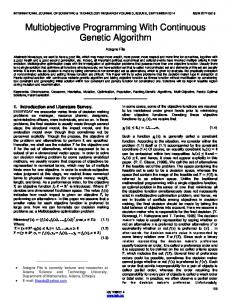
4.1. One-pipe pumping system (Case 1) Figure 4a shows a simple one-pipe pumping system, which consists of a lower reservoir (water source), one pump, one rising main and an upper reservoir. The design conditions are summarised in Table 4. The aim of the design is to select the best combination of the pump size and the pipe size that can deliver the minimum average peak-day flow and also minimise both the total cost and GHG emissions of the network during its design life. Thirty different fixed speed pumps and twenty-six DICL pipes of different diameters are considered as options in this study. The pumps were selected using Thompson Kelly & Lewis’ pump selection program EPSILON. The prices of the pumps and corresponding pump stations are calculated according to the sizes of the pumps. The unit weights of the pipes are calculated according to the DICL pipe data obtained from Tyco Water. Details of the pipes are given in Table 3 in the previous section; and the details of pumps are given in Table 5.
(a)
(b)
Figure 4 One-pipe pumping system ((a) System configuration; (b) Trade-off curves for the rank 1, rank 2 and rank 3 solutions) This system was optimised using both single-objective (considering cost) and multi-objective (considering cost and GHG emissions) methods. An average electricity tariff of 13.5 cents per kWh was used. For the multi-objective optimisation runs, each objective was discounted using the same method - either single rate discounting or Gamma discounting. A typical discount rate of 8% obtained from SA Water was used for single rate discounting. The results obtained from both single-objective and multi-objective optimisations are summarised in Tables 6 and 7, respectively. It is evident from Tables 6 and 7 that, as expected, the single-objective optimisation only found one solution – the minimum cost solution. However, in the multi-objective optimisation using Gamma discounting, two other non-dominated solutions were found. This gives three Pareto-optimal solutions
WATER DOWN UNDER 2008 Wu, Simpson, Maier
7 of 12
MOGA Optimisation of WDSs Accounting for Sustainability
Wu
in total. Table 7 shows that when a single discount rate of 8% is used, the number of Pareto-optimal solutions is reduced to two, as a larger 450 mm pipe and the corresponding pump are not selected. This is because a single large discount rate takes away the advantage of larger pipes by reducing the effects of the impacts the system has on the environment in the future. This can be explained by comparing the present values of annual pumping cost and GHG emissions obtained using a single discount rate of 8% and those obtained using Gamma discounting. Table 8 shows the comparison of these results. When a single discount rate of 8% is used, the present values of both future annual th pumping cost and GHG emissions decline quickly and finally reach zero or near zero at the 100 year. However, when Gamma discounting is used, the present values decline more slowly; therefore, the economic impact and the impact the system has on the environment at the end of the design life are also taken into account. Table 4 Design conditions of case 1 Annual demand (m3) Average peak-day flow (L/s) Static head (m) Pipe length (m) Design life (years)
1,500,000 120 95 1,500 100
Table 5 Pump information and pump station costs No. Pump Type/Size Speed (rpm) Dia (mm) 1 EC/8*17A_ECS 1475 410 2 EC/8*17A_ECS 1475 432 3 EC/8*17B 1475 393 4 EC/8*17B 1475 445 5 EC/8*17B_ECS 1475 445 6 HN/8HN124A 2950 293 7 HN/8HN124A 2950 318 8 LR/6LG13/A 2900 311 9 LR/6LG13/A 2900 321 10 VDP/430DMH 1480 251 11 VDP/430DMH 1480 275 12 VDP/430DMH 1480 312 13 VDP/430DMH 1480 312 14 VDP/430DML 1480 272 15 VDP/430DML 1480 290 16 VDP/430DML 1480 313 17 VDP/430DML 1480 313 18 VDP/460CDKH 1480 280 19 VDP/460CDKH 1480 336 20 VDP/460DKL 1480 295 21 VDP/460DKL 1480 334 22 VDP/460DKL 1480 336 23 VDP/510DML 1480 332 24 VDP/510DML 1480 369 25 VDP/510DMH 980 339 26 VDP/510DMH 980 368 27 SUPER-TITAN/200*300-630 1480 537 28 SUPER-TITAN/200*300-630 1480 635 29 SUPER-TITAN/250*300-500B 1480 553 30 SUPER-TITAN/250*300-500B 1480 562 *BEP: Best Efficiency Point **In this study, all monetary costs are in Australian dollars.
BEP* (%) 83.1 83.3 81.7 84 84 78.5 81 80.4 80.8 83.3 84 85 85 81.3 81.6 81.9 81.9 81.3 83 84.2 85.1 85.2 79.5 81.2 83.3 83.2 81.3 82.8 84.2 84.3
Motor (kW) 185 225 185 260 185 225 300 185 225 185 185 260 335 185 185 225 260 225 375 185 185 260 260 335 225 300 300 450 335 375
Price ($)** 1,092,239 1,235,213 1,092,239 1,348,458 1,092,239 1,235,213 1,466,297 1,092,239 1,235,213 1,092,239 1,092,239 1,348,458 1,560,763 1,092,239 1,092,239 1,235,213 1,348,458 1,235,213 1,660,459 1,092,239 1,092,239 1,348,458 1,348,458 1,560,763 1,235,213 1,466,297 1,466,297 1,828,954 1,560,763 1,660,459
Table 6 Single-objective optimisation results for Case 1 (Gamma discounting) No. 1
Pump 5
Pipe Dia. (mm) 300
Flow (L/s) 120.17
WATER DOWN UNDER 2008 Wu, Simpson, Maier
Efficiency (%) 83.1
Cost (M$) 5.83
GHG (ton) 20,172
8 of 12
MOGA Optimisation of WDSs Accounting for Sustainability
Wu
Table 7 Multi-objective optimisation results for Case 1 Rank Single discount rate of 8%
1
Gamma Discounting
1
No.
Pump
Pipe Dia. (mm)
Flow (L/s)
1 2 1 2 3
5 5 5 5 11
300 375 300 375 450
120.17 134.75 120.17 134.75 149.50
Annual pumping hours 3467 3092 3467 3092 2787
Efficiency (%)
Cost (M$)
GHG (ton)
83.1 83.6 83.1 83.6 83.5
3.15 3.44 5.83 5.98 6.25
8,284 8,124 20,712 19,490 19,461
Table 8 Comparison of discounting results of design No. 1 for Case 1 Single discount rate of 8%
Gamma discounting
Year
PV of Annual Pumping Cost (M$)
PV of Annual GHG (ton)
PV of Annual Pumping Cost (M$)
PV of Annual GHG (ton)
1 5 6 25 26 75 76 100
0.0671 0.0493 0.0457 0.0106 0.0098 0.0002 0.0002 0.0000
518.13 380.84 352.63 81.71 75.66 1.74 1.61 0.25
0.0697 0.0596 0.0579 0.0330 0.0323 0.0123 0.0121 0.0096
538.05 459.93 446.54 254.65 249.66 94.61 93.67 73.77
Table 9 Results from full enumeration for Case 1 Rank 1
2
3
No. 1 2 3 4 5 6 7 8 9
Pump 5 5 11 1 5 10 11 14 20
Pipe Dia. (mm) 300 375 450 300 450 375 375 300 450
Flow (L/s) 120.17 134.75 149.5 120.19 139.25 138.02 141.42 120.26 148.06
Efficiency (%) 83.1 83.6 83.5 82.5 83.2 82.8 82.5 81.0 83.4
Cost (M$)
GHG (ton)
5.83 5.98 6.25 5.85 6.25 6.01 6.03 5.90 6.25
20,712 19,490 19,461 20,858 19,465 19,721 19,842 21,221 19,481
In addition, a full enumeration with Gamma discounting was carried out for this system, in which all 780 possible solutions were evaluated and ranked. The details of the top three ranked solutions of the system from full enumeration are summarised in Table 9. A plot of these solutions is presented in Figure 4b. The results of the full enumeration show that there are three Pareto-optimal solutions in the entire search space when Gamma discounting is used. Therefore, the multi-objective genetic algorithm developed has found all of the Pareto-optimal solutions to this problem. In a parametric study, a number of GA runs were carried out with population sizes of 10, 20, 30 and 50, a crossover probability of 0.9 and ten mutation probabilities ranging from 0.05 to 0.5. The numbers of evaluations that were required to find all three Pareto-optimal solutions ranged from 140 to 400. However, for a multi-objective optimisation problem, in addition to the number of evaluations, the number of comparisons is also important in determining the computational effort in obtaining the desired results. This is because even though each of the comparisons takes less time than an objective function evaluation, the number of comparisons required by the non-dominated sorting used in a multiobjective algorithm is much larger. According to Deb et al. (Deb, et al., 2002), the maximum computational complexity of the current non-dominated sorting method used in this study to find the 2 Pareto-optimal front or the first non-dominated front is O(MN ), where M is the number of objectives 2 and N is the number of solutions. For this case study, M*N =2*780*780=1,216,800 comparisons could be required. The number of comparisons used for the MOGA to find all three Pareto-optimal solutions in the parametric study ranged from 4,000 to 150,000, which is 0.33% to 12.3% of the comparisons that would be required if the search space were ranked in order to find the values that define the Pareto optimal front. Therefore, the use of multi-objective optimisation is still very efficient, even for a problem with such a relatively small search space.The plot of the Pareto-optimal front (Figure 4b) shows significant trade-offs between the economic and environmental objectives. When the total cost
WATER DOWN UNDER 2008 Wu, Simpson, Maier
9 of 12
MOGA Optimisation of WDSs Accounting for Sustainability
Wu
of the system is increased from $5.83 M for design 1 to $5.98 M for design 2, GHG emissions are reduced from 20,712 tonnes to 19,490 tonnes. This is a 5.90% reduction in GHG emissions by only increasing the total cost of the system by 2.57%. However, in order to get a further 0.15% reduction in GHG emissions (from design 2 to design 3), a 4.52% increase in cost is required.
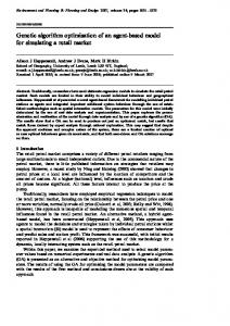
4.2. Multi-pump system (Case 2) Figure 5a shows the system configuration of the second case study. In this case study, a typical WDS consisting of a source of potable water (reservoir), a main pump, a rising main, a booster pump, a transmission main and a tank needs to be designed. There are two possible tank locations: A and B. Therefore, there are five decision variables: the size of the main pump (pump 1), the size of the rising main (pipe1), the location of the tank (A or B), the size of the corresponding pump (pump 2 or 3) and the size of the corresponding transmission main (pipe 2 or 3). The design conditions of this system are summarised in Table 10. It should be noted here that the elevation of tank A is higher than that of tank B, which gives tank A an advantage over tank B in distributing water to networks downstream of the tanks. However, this advantage is not considered in this case study. The available pumps and pipes are the same as those in case study 1. This system was optimised accounting for only the cost first, and then accounting for both cost and GHG emissions. An average electricity cost of 13.5 cents per kWh and Gamma discounting were also used. Similar to the first case study, for the multi-objective optimisation, both objectives were discounted using Gamma discounting in each GA run. The optimisation results are summarised in Table 11.
(a)
(b)
Figure 5 Multi-pump system ((a) System configuration; (b) Pareto-optimal solutions) Table 10 Design conditions of Case 2 Annual demand (m3) Average peak-day flow (L/s) Design life (year)
1,500,000 120 100
Pipe 1 length (m) Pipe 2 length (m) Pipe 3 length (m)
30,000 15,000 20,000
Table 11 Optimisation results for Case 2
Singleobjective Multiobjective
No.
Tank
1 2 1 2 3 4
A A A A A A
No. of Pump 1 13 4 13 4 4 4
Pipe 1 Dia. (mm) 375 375 375 375 375 450
No. of Pump 2 4 13 4 13 4 5
Pipe 2 Dia. (mm) 375 375 375 375 450 375
Flow (L/s) 125.28 125.28 125.28 125.28 127.43 120.52
Eff.1 (%) 77.3 83.7 77.3 83.7 83.8 83.3
Eff. 2 (%) 83.7 77.3 83.7 77.3 83.8 83.3
Cost (M$) 51.23 51.23 51.23 51.23 53.10 54.94
GHG (ton) 114,280 114,280 114,280 114,280 111,573 109,392
The single-objective optimisation results show that there are two minimum cost solutions, which both cost $51.23 M in present value terms over the 100-year design life. Ten runs were carried out for the multi-objective optimisation. Two other non-dominated solutions were found in two of the ten runs. In
WATER DOWN UNDER 2008 Wu, Simpson, Maier
10 of 12
MOGA Optimisation of WDSs Accounting for Sustainability
Wu
eight other runs, no other non-dominated solutions were found. A full ranking of all enumerated solutions of this system is not feasible, because for this problem, where there are 1,216,800 possible 2 solutions, 2.96E+12 comparisons (MN ) could be required to find the Pareto-optimal front only. This would take about 2.5 years on a typical PC. In order to show the position of the Pareto-optimal front, the total 1,216,800 solutions were fully enumerated and the top 100 low cost solutions and top 100 low GHG emission solutions were plotted in Figure 5b, together with the Pareto-optimal solutions. Figure 5b shows that the top 100 low cost solutions and top 100 low GHG emission solutions form four groups of solutions. The Pareto-optimal front spans the best solutions in three of the four groups. In addition, the front shows significant trade-offs between the economic and environmental objectives. From design 1 and 2 to design 3, a 3.65% increase in cost leads to a 2.37% reduction in GHG emissions. From design 3 to design 4, a 3.47% increase in cost leads to a further 1.95% decrease in GHG emissions, which means that a 7.24% increase in cost resulted in a reduction of 4.28% in GHG emissions in total. Therefore, all of four designs are possible solutions to this problem in terms of both criteria.
5. CONCLUSIONS This paper introduces a multi-objective approach for solving the WDS design problem, accounting for both economic and environmental objectives. A multi-objective genetic algorithm was developed based on a well known multi-objective genetic algorithm (NSGA-II) and an efficient constraint handling method (constrained tournament selection). The impact that minimising GHG emissions has on the results of WDS optimisation has been explored for two simple case studies: a one-pipe pumping system and a multi-pump system. In addition, results obtained from optimising WDSs accounting for both economic and environmental objectives are compared with those obtained when only a single economic objective was considered. The comparison of the results indicates that the inclusion of GHG emission minimisation as one of the objectives results in significant tradeoffs between the economic objective and the environmental objective. In both of the case studies, a reasonable increase in the cost results in a substantial reduction in GHG emissions. Furthermore, the impacts of Gamma discounting on present value analysis were investigated by comparing the results obtained from calculating present values using a single discount rate to those obtained from using Gamma discounting for the first case study. A comparison of the results shows that a high single discount rate eliminates the advantage of larger pipes by reducing the effects of the impact the system has on the environment in the future, whereas, Gamma discounting places relatively more weight on the future effects compared to a single discount rate of 8% that is typically used by water utilities. In conclusion, the minimisation of GHG emissions has been incorporated into the optimisation of the design of WDSs as the second objective for the first time in this study. The multi-objective optimisation approach used in this paper provides the designer with more alternatives resulting from the conflicting objectives and therefore allows the designer to choose one solution by considering the tradeoffs between two criteria. The time value of both cost and GHG emissions have been taken into account by using present value analysis and Gamma discounting was used to calculate the present value of both the future monetary costs, and GHG emissions resulting from the operation of the system. The values of discount rates have significant impacts on the results of present value analysis. Therefore, it is important to explore the sensitivity of changes in marginal discount rates assumed for both the economic and environmental objectives of WDS optimisation in the future.
6. ACKNOWLEDGEMENT The authors would like to thank the reviewers for their comments which helped to improve the paper.
7. REFERENCES Ambrose, M. D., Salomonsson, G. D. and Burn, S. (2002), Piping Systems Embodied Energy Analysis, CMIT Doc. 02/302, CSIRO Manufacturing and Infrastructure Technology, Highett, Australia.
WATER DOWN UNDER 2008 Wu, Simpson, Maier
11 of 12
MOGA Optimisation of WDSs Accounting for Sustainability
Wu
Australian Greenhouse Office (2006), AGO Factors and Methods Workbook, Canberra. Bagamery, B. D. (1991), Present and Future Values of Cash Flow Streams: The Wristwatch Method, Financial Practice & Education, Vol.1(2), pp. 89-92. Bazelon, C. and Smetter, K. (2001), Discounting in the Long Term, Loyola of Los Angeles Law Review, Vol.35(277). Dandy, G. C. and Hewitson, C. (2000), Optimising Hydraulics and Water Quality in Water Distribution Networks using Genetic Algorithms, Joint Conference on Water Resources Engineering and Water Resources Planning and Management, (Ed, ASCE), Minneapolis. Dandy, G. C., Roberts, A., Hewitson, C. and Chrystie, P. (2006), Sustainability Objectives for the Optimization of Water Distribution Networks, Proceedings of 8th Annual Water Distribution Systems Analysis Symposium, Cincinnati, USA Deb, K. (2000), An efficient constraint handling method for genetic algorithms, Comput. Methods Appl. Mech. Engrg., Vol.186 pp. 311-338. Deb, K. (2002), Multi-objective Optimization using Evolutionary Algorithms, John Wiley & Sons, Ltd, West Sussex, England. Deb, K., Pratap, A., Agarwal, S. and Meyarivan, T. (2002), A Fast and Elitist Multi-Objective Genetic Algorithm: NSGA-II, KanGAL, India Institute of Technology Kanpur, Kanpur, India. Filion, Y. R., MacLean, H. L., A.M., A., Karney, B. W. and ASCE M. (2004), Life-Cycle Energy Analysis of a Water Distribution System, Journal of Infrastructure Systems, Vol.10(3). Foley, B. A. and Daniell, T. M. (2002), A Sustainability tool for intrasectoral and intersectoral water resources decision making, The 27th Hydrology and Water Resources Symposium, Melbourne, Australia Ghimire, S. R. and Barkdoll, B. D. (2007), Incorporating Environmental Impact in Decision Making for Municipal Drinking Water Distribution Systems Through Eco-Efficiency Analysis, Proceedings of the World Environmental and Water Resources Congress 2007: Restoring Our Natural Habitat, (Ed, Kabbes, K. C.), Tampa, Florida Gilman, R. (1992) IN CONTEXT: A Quarterly of Humane Sustainable Culture, Vol., Context Institute, http://www.context.org/ICLIB/DEFS/AIADef.htm, [Accessed online: 19 May 2007] Goldberg, D. E. (1989), Genetic Algorithm in Search Optimization, and Machine Learning, AddisonWesley Publishing Company, Inc., Canada. Hu, X. (1997), Sustainability of Effluent Irrigation Schemes: Measurable Definition, Journal of Environmental Engineering, pp. 928-932. Kaen, F. R. (1995), Corporate Finance, Blackwell Business, USA. Keedwell, E. and Khu, S.-T. (2006), A novel evolutionary meta-heuristic for the multi-objective optimization of real-world water distribution networks, Engineering Optimization, Vol.38(3), pp. 319-336. Prasad, T. D. and Park, N.-S. (2004), Multiobjective Genetic Algorithms for Design of Water Distribution Networks, Journal of Water Resources Planning and Management, Vol.130(1), pp. 73-82. Sahely, H. R., Kennedy, C. A. and Adams, B. J. (2005), Developing sustainability criteria for urban infrastructure systems, Canadian Journal of Civil Engineering, Vol.32(1), pp. 72-85. Sarbu, I. and Borza, I. (1998), Energetic optimization of water pumping in distribution systems, Mechanical Engineering, Vol.42(2), pp. 141-152. Savic, D. (2002), Single-objective vs. Multiobjective Optimisation for Integrated Decision Support, Proceedings of the First Biennial Meeting of the International Environmental Modelling and Software Society, (Eds, Rizzoli, A. E. and Jakeman, A. J.), Lugano, Switzerland pp. 7-12 Simpson, A. R., Dandy, G. C. and Murphy, L. J. (1994), Genetic algorithms compared to other techniques for pipe optimization, Journal of Water Resources Planning and Management, Vol.120(4), pp. 423-443. Trelor, G. J. (1994), Energy Analysis of the Construction of Office Buildings, Master of Architecture Thesis, Deakin University, Geelong. Weitzman, M. L. (2001), Gamma Discounting, The American Economic Review. Zecchin, A. C., Simpson, A. R., Maier, H. R., Leonard, M., Roberts, A. J. and Berrisford, M. J. (2006), Application of two ant colony optimisation algorithms to water distribution system optimisation, Mathematical and Computer Modelling, Vol.44(5-6), pp. 451-468.
WATER DOWN UNDER 2008 Wu, Simpson, Maier
12 of 12