constraint and their satisfaction degrees by (fc1 ءءء fcn) and. ( 1 ءءء n), respectively. The corrective values for updating the control input and the final time are ...
Trans. Japan Soc. Aero. Space Sci. Vol. 47, No. 155, pp. 66–74, 2004
Multi-Objective Trajectory Optimization by a Hierarchical Gradient Algorithm with Fuzzy Decision Logic —Application to Slew Maneuver Problems of a Flexible Space Structure— By Hirohisa KOJIMA and Nobuyuki N AKAJIMA Department of Aerospace Engineering, Tokyo Metropolitan Institute of Technology, Hino, Japan (Received September 5th, 2003)
The rest-to-rest maneuver problem of a flexible space structure is a two-point boundary value problem (TPBVP) and is solved by some gradient methods. If TPBVP is strongly restricted by constraints, TBVP becomes an ill-defined problem, and the solution meeting all constraints cannot be obtained. However, reasonable suboptimal solutions are often needed since real plant systems are necessary to be controlled. In order to obtain such suboptimal solutions, we have developed a modified version of the hierarchy gradient method by installing fuzzy decision logic. Constraints are classified into non-fuzzy constraints and fuzzy constraints according to their priorities. Fuzzy constraints having a trade-off relationship with each other are compromised reasonably by fuzzy decision logic. The usefulness of the proposed method is numerically and experimentally verified by applying it to the rest-to-rest slew maneuver problem of a flexible space structure, where fuzzy constraints are final time, sensitivity of residual vibration energy with respect to the structure frequency uncertainty and maximum bending moment at the root of the flexible appendage. Key Words:
1.
Optimal Control, Gradient Algorithm, Fuzzy Decision, Slew Maneuver, Flexible Space Structure
Introduction
The control of the vibration and attitude of a flexible space structure is important in space engineering. Numerous research based on the unique characteristic of flexible space structures has been carried out. The time optimal control problem for flexible space structures is one example of such research; various methods for suppressing vibration of flexible space structures have been proposed1–16) and experiments were carried out.17–19) Singhose et al.,10,11) Singer and Seering12) and Rogers and Seering13) have studied the input shaping method, which is the open-loop control method and does not induce vibration on flexible space structures much by using a frequency shaped command. Singhose11) has also proposed the method that not only minimizes maneuver time, but also restrains the deflection of the flexible appendage under a considered value in order to suppress the load affecting the flexible appendage during maneuver. We have proposed a minimum bendingmoment control (MBMC) method in which the maximum value of the bending moment induced on the root of the flexible appendage is restricted (in addition, the L2 norm of the bending-moment is minimized during maneuver), and experimentally verified the validity of the method.20) The optimal control input to flexible space structures can be obtained by maximizing or minimizing the evaluation function while satisfying the various constraint conditions. Optimal control problems are not always well defined because there are cases where constraint conditions having a trade-off relationship with each other are sometimes too reÓ 2004 The Japan Society for Aeronautical and Space Sciences
stricted and the solution satisfying all conditions cannot exist. Conventional algorithms cannot derive optimal control input for such ill-defined problems mathematically because they have been developed to solve the well-defined optimal control problem in which the solution satisfying all the constraint conditions exists. Even if constraints on control inputs and state variables are severe and a solution satisfying all constraints cannot be found, we need to obtain various suboptimal solutions by mitigating constraints in accordance with certain judgment standards, because real systems need to be controlled by some reasonable solutions. In order to obtain some reasonable solutions, various methods such as adding a penalty function to the evaluation function21) and composing the evaluation function with the linear shape sum of a plural constraint condition22) are often carried out. However, it is hard to predict the relationship between the coefficient of the penalty function and resulting solutions, and there is not conclusive evidence that the obtained solution reflects the designer’s demands accurately. Suzuki and Yoshizawa23) have applied a goal programming method to obtain a suboptimal solution that meets the designer’s demands, even if the problem is ill defined, by setting a goal value for each constraint and evaluation function, and by making a priority order of them. They have also shown that the goal programming method can be applied to a case where the order of priority among constraints cannot be specified distinctly, by using fuzzy decision logic. Their method, however, needs discrete state variables in order to transform the problem into a linear programming problem, and this transformation gives rise to a drawback that an accurate solution might not be obtained.
May 2004
H. KOJIMA and N. N AKAJIMA: Multi-Objective Trajectory Optimization by a Hierarchical Gradient Algorithm
To overcome this problem in Suzuki’s method, we focus on the hierarchical gradient method,24) which can solve the optimal control problem with plural constraints, and an accurate evaluation function because this algorithm does not need discrete state variables. This method is formulated as follows: first, a priority is made among the constraints, and the gradient of the control input profile is calculated so that the prioritized constraint is satisfied. Then, the null-vector space of the resulting gradient, which does not disturb the satisfaction of the prioritized constraints, is utilized to satisfy the lower level constraints and to minimize the performance index. This scheme cannot, however, treat the ill-defined problem in which the classification of priority is not clearly defined since this algorithm assumes that the constraints are completely satisfied. The following improvement of this algorithm is presented to obtain the solution of such ill-defined problems. First, the hierarchical gradient method is modified so that the final time of the optimal control problem can be treated as a parameter to be optimized. Second, each constraint condition and the evaluation function are classified into non-fuzzy constraints or fuzzy constraints in accordance with those orders of priority, and the achievement degrees of fuzzy constraints are expressed with the membership functions. Then, the control input profile and final time are updated in each iteration step, taking the values of the membership functions into consideration. As the result of this process, the suboptimal solution satisfying equally the fuzzy constraints is obtained without disturbing the convergence of the non-fuzzy constraint. The multi-objective trajectory optimization problem of a flexible space structure, in which the solution satisfying all constraints does not exist, is studied, and the efficacy of the hierarchical gradient method with fuzzy decision logic is verified experimentally by implementing the obtained control input profile to the rest-to-rest slew maneuver problem of a flexible space structure. 2.
2.1.
Hierarchical Gradient Method with Fuzzy Decision Logic
Improvement of the hierarchical gradient method to treat the time optimal control problem Several methods for solving the two-point boundary problem have been proposed. In the present study, we use the hierarchical gradient method to solve the optimal control problem. In this method, null-space vectors of the equation of constraints on the state variables at the final time are used to satisfy the inequality constraint on the state variables. Thus, the hierarchical gradient method can be expected to be robust with respect to the inaccuracy of the initial estimation for the control input profile. The original hierarchical gradient method can treat neither the constraint on the value of the control input nor the time-optimal control problem. In this subsection, we briefly explain a modified version of the method to overcome such drawbacks of the original algorithm. See the process of derivation described in the Appendix and refer to Ref. 24).
67
2.1.1. Problem formulation In order to enable the hierarchical gradient method to treat the time-optimal control problem, the time scale is normalized so that the fictitious final time becomes 1 as t ¼ p�, p ¼ tf (0 � � � 1). After the time scale transformation, the optimal control problem is rewritten as follows: x0 ¼ f ðx; u; �; pÞp;
Equation of motion (Rn ):
Constraints at the initial time (Rn ):
ð1Þ
xð0Þ ¼ x0 ;
ð2Þ
c1
Constraints at the final time ðR Þ: c1 ðxð1Þ; pÞ ¼ 0; c2
Constraints on the state variables (R ): Z
ð3Þ
gðxÞ � 0;
ð4Þ
1
Minimize J ¼
Lðx; u; �; pÞpd�;
ð5Þ
0
where the overdash denotes the differential with respect to the fictitious time, �, and Eq. (1) corresponds to the equation of motion. Hereafter, we refer to Eq. (3) as the final constraint and Eq. (4) as the state constraint. Since the inequality constraint on the state variables cannot be easily treated in an algorithm that calculates the gradients of both the constraint and the performance index with respect to all state variables for solving the two-point boundary value problem, such a constraint needs to be converted to an equality constraint. We will explain this conversion in the following subsection. 2.1.2. Conversion of inequality constraint to equality constraint Let us consider the following function: Z1 c2 ¼ dðxð�ÞÞpd�; ð6Þ 0
�
where dðxÞ ¼
dðxÞ > 0 0
if gðxÞ > 0 if gðxÞ � 0.
ð7Þ
If the inequality constraint is satisfied, c2 becomes zero. Therefore, we can substitute the equality constraint, c2 ¼ 0 for the inequality constraint of Eq. (4). 2.1.3. Updating control input profile and final time by the hierarchical gradient method A corrective value of control input and final time in the hierarchical gradient method consists of three elements; an element to satisfy the final condition, an element to satisfy the state constraint, and an element to reduce the performance index. We now describe each element. (1) Element to satisfy the final condition �uð�Þ ¼ �W1u ð�Þ�ð�ÞD�1 11 c1 þ �y1 ð�Þ �Z 1 � T �1 D11 W1u ð�Þ�y1 ð�Þdt þ W1p ð0Þ�y2 ; � W1u 0
ð8Þ �p
T ð0ÞD�1 ¼ �W1p 11 c1 þ �y2 �Z 1 T �1 � W1p D11 W1u �ð�Þ�y1 ð�Þd� 0
� þ W1p ð0Þ�y2 ; ð9Þ
68
Trans. Japan Soc. Aero. Space Sci.
where �y1 and �y2 are null space vectors with respect to Eq. (33) (that is an equation to determine corrective values of control input and final time to satisfy the final constraints), and corrective values of control input and final time, respectively, to satisfy the state constraint, as shown in the following paragraph. Parameter � is an arbitrary negative constant. Regarding other variables such as �ð�Þ, W1u and W1p , refer to the Appendix for their definitions. (2) Element to satisfy the state constraint Without affecting the convergence of the final constraint, arbitrary corrective values for �y1 and �y2 can be chosen as follows: �1 �y1 ð�Þ ¼ �W^ 2u ð�Þ�ð�ÞD�1 22 ðc2 � D21 D11 c1 Þ þ �z1 ð�Þ �Z 1 T � W^ 2u W^ 2u ð�Þ�ð�Þ�z1 ð�Þd� ð�Þ�ð�ÞD�1 22
ð10Þ
T �1 ð�ÞD�1 �y2 ¼ �W^ 2p 22 ðc2 � D21 D11 c1 Þ þ �z2 �Z 1 T W^ 2u ð�Þ�ð�Þ�z1 ð�Þd� � W^ 2p ð0ÞD�1 22
1 0
Hu ð�ÞHuT ð�Þd� þ �Vp ð0ÞVpT ð0Þ � 0: ð16Þ
Thus, we can expect that the performance index converges in the iteration of the hierarchical gradient algorithm. The corrective values for the control input and the final time by combining the above three elements are finally obtained as follows: T �1 �uð�Þ ¼ �W1u ð�Þ�ð�ÞD�1 11 c1 þ �Ku ð�Þðc2 � D21 D11 c1 Þ T ð�Þ�ð�ÞD�1 þ �HuT ð�Þ � �W1u 11 Z1 � W1u ð�Þ�ð�ÞHuT ð�Þd� 0
ð11Þ
ð12Þ
where H is a Hamiltonian defined as Hð�Þ ¼ Lðx; u; �; pÞp þ �ð�Þf ðx; u; �; pÞp;
ð13Þ
� is a costate vector, and v1 and v2 are Lagrangian multipliers for the final constraint and the state constraint, respectively. When the constraints have converged sufficiently, the first variation of the extended performance index with respect to both the control input and the final time, the corrective value of the control input, and the final time can be approximated, respectively, as follows: Z1 � �J � Hu ð�Þ�ud� þ Vp ð0Þ�pð0Þ; 0
�p � z2 :
ð14Þ
If values z1 and z2 are chosen as follows: �z2 ¼ �Vp ð0Þ ð� < 0; � < 0Þ
1
W^ 2u ð�Þ�ð�ÞHuT ð�Þd�
� �Ku ð�Þ 0
T �1 � �Ku ð�ÞW^ 2p ð0ÞVp ð0Þ � �W1u D11 ð0ÞVp ð0Þ; ð17Þ T �1 ð0ÞD�1 �p ¼ �W1p 11 c1 þ �Kp ð0Þðc2 � D21 D11 c1 Þ Z1 T �1 þ �Vp ð0Þ � �W1p ð0ÞD11 W1u ð�Þ�ð�ÞHuT ðtÞdt
0
0
1
W^ 2u ð�Þ�ð�ÞHuT ð�Þd�
� �Kp ð0ÞW^ 2p ð0ÞVp ð0Þ
0
þ ðv1 c1 þ v2 c2 Þ;
Z
� �Kp ð0Þ
where �z1 and �z2 are null space vectors with respect to Eq. (34) (that is an equation to determine corrective values of control input and final time to satisfy the state constraint). (3) Element to reduce the performance index The parameter p is independent of the imaginary time, �. Thus, we can introduce the following function as the extended performance index in the present study: Z1 � J ¼ ðHð�Þ � �p p0 ð�Þ � �x x0 Þ�ud�
�z1 ¼ �HuT ;
Z
Z
0
þ W^ 2p ð0Þ�z2 ;
�u � z1 ;
�J � � �
0
� ^ þ W2p ð0Þ�z2 ;
�
Vol. 47, No. 155
ð15Þ
then the first variation of the extended performance index (Eq. (14)) becomes approximately negative
T �1 D11 W1p ð0ÞVp ð0Þ: � �W1u
ð18Þ
2.2. Fuzzy decision logic While the hierarchical gradient method was improved to treat the time optimal control problem, the method still cannot be applied to the ill-defined problem including prioritized and nonprioritized constraint conditions. In other words, the method fails to obtain the solution reflecting the designer’s intention that can be represented in the form of a fuzzy decision. We show a method to combine the hierarchical gradient method with the fuzzy decision logic so that a reasonable solution reflecting the designer’s intention can be obtained, even if the problem corresponds to the illdefined problem in the present paper. First, each constraint condition and evaluation function are classified into non-fuzzy constraints and fuzzy constraints in accordance with their priority. The non-fuzzy constraints are treated as constraints that must be satisfied as much as possible first, and the satisfaction degrees of the fuzzy constraints are raised as much as possible without interfering with the convergence of the non-fuzzy constraints. This process can be conducted in the hierarchical gradient method by utilizing the null space vector of equations of non-fuzzy constraints for raising the satisfaction of the fuzzy constraints. In order to represent the satisfaction degree of each fuzzy constraint, membership functions are designated. The value of the membership function is zero when the value of the evaluating item is worse than or equal to the worst possible case, and has a value of one when the value of the item is better than or equal to the best possible case, and has an intermediate value for the case between the best and worst cases. Any type of membership function can
May 2004
H. KOJIMA and N. N AKAJIMA: Multi-Objective Trajectory Optimization by a Hierarchical Gradient Algorithm
be employed and designers can express their design demands in the form of the membership function. Let us denote sets of membership functions of the fuzzy constraint and their satisfaction degrees by ( fc1 � � � fcn ) and (�1 � � � �n ), respectively. The corrective values for updating the control input and the final time are calculated in the hierarchical gradient algorithm with fuzzy decision logic as follows: If �i is minimum among (�1 � � � �n ) then � � uðtÞ � ¼ the corrective values p to satisfy the non-fuzzy constraints þ the corrective value to increase �i :
ð19Þ
Consequently, the optimal solution can be obtained with equal satisfaction degrees among fuzzy constraints and without disturbing the satisfaction of the non-fuzzy constraints. 3.
Flexible Space Structure
3.1. System model Illustrated in Fig. 1 is a model of a space structure consisting of a rigid body equipped with a flexible appendage. The appendage is a cantilever beam with one end fixed to the rigid body and the other end free. Translational and vibrational motions are assumed to be planar two-dimensional motion. We assume that the control input is applied only on the rigid body. Neglecting the structural damping and the air drag, the behavior of the present model is described by the following equations of motion: Zl 2 @ y1 ð ; tÞ ðm0 þ �lÞy€0 ðtÞ þ � d ¼ uðtÞ ð20Þ @t2 0 �y€0 ðtÞ þ �
@2 y1 ð ; tÞ @4 y1 ð ; tÞ þ EI ¼0 2 @t @ 4
ð21Þ
with the boundary conditions:
ξ Displacement
y1 (ξ,t) Flexible Beam
69
@y1 ¼ 0 at ¼ 0; @ @2 y1 @3 y1 ¼ 3 ¼ 0 at ¼ l @2 @ y1 ¼
ð22Þ
where the dot indicates differentiation with respect to time, y0 denotes the displacement of the rigid body, u is the control input, and m0 , � and EI denote the mass of the rigid body, the mass density of the beam per unit length and the bending rigidity of the beam, respectively. The parameters � and EI are assumed to be constant along the beam. Expanding the flexible vibration of the appendage by vibrational modes, and transforming the state variable using an appropriate transformation matrix, Eqs. (20) and (21) can be rewritten in the following state-space equation: x_ðtÞ ¼ AxðtÞ þ BuðtÞ;
ð23Þ
where x, A and B are, respectively, x ¼ ½x0 x_0 q1 q_1 � � � qi q_i � � � qn q_n �T ;
ð24Þ
A ¼ blockdiag ½A0 � � � Ai � � � An �; " # " # 0 1 0 1 ; Ai ¼ A0 ¼ ; 0 0 �!2i 0
ð25Þ ð26Þ
B ¼ ½0 0 0 1 � � � 0 i � � � 0 n �T ;
ð27Þ
A0 and Ai are the matrix associated with the rigid body motions and the i-th modal matrix, respectively, and qi , i and !i are the i-th flexible modal displacement, the i-th modal gain, and the i-th flexible modal frequency, respectively. In the present study, we consider only the first modal vibration on the beam to simplify the analysis. 3.2. Experimental setup The system parameters for the experiment are listed in Table 1. Figure 2 shows the apparatus of the experimental setup. The model of the flexible appendage is a 0.96 m long aluminum beam clamped to the rigid body. Two full-bridge strain gauges are located at the root of the beam to measure the bending moment there. A signal from the gauges is amplified and recorded in a computer, using a sampling time of 0.003[sec]. The rigid body moves in a horizontal plane through actuation of a linear motor. Since the linear motor employed in this study cannot be operated by force control but only by velocity control, the velocity-based control is employed to actuate the rigid body. The position of the rigid body is sensed through the incremental encoder and the velocity of the rigid body is compensated to follow the reference velocity by feeding the torque to the motor according
Bending-Moment
Table 1. System parameters.
M(0,t) Control Input
y0 (t)
Main Body
Fig. 1. Model of a flexible space structure.
u(t)
Weight of the main body
m0
14.0 kg
Length of the beam
l
0.96 m
Bending stiffness
EI
1.01 Nm
Unit weight of the beam
�
0.128 kg/m
Final position of the main body
y0f
2.0 m
Maximum control input
umax
50.0 N
70
Trans. Japan Soc. Aero. Space Sci.
It can be expected that the residual vibration that has the frequency between !1 and !2 becomes small even if the actual frequency is different from the nominal one when this value is small. The frequency of the experimental model is 8.69 rad/s. In the present study, the integral range is chosen between plus and minus 30% of this value, (!1 ¼ 6:08 rad/s, !2 ¼ 11:29 rad/s), for evaluating the robustness. The analysis result and the experiment result are shown for each case in the following subsections. 4.1. CASE-1 In this case, the demands having the trade-off relationship with each other are to suppress the maximum value of the bending moment induced at the root of the beam and to move a specified distance as fast as possible. Let us denote the satisfaction degrees of the final time and the maximum value of the bending moment at the root of the beam by �1 and �2 , respectively. The optimal control problem is formulated as follows:
Amplifier
Strain gauges PC
Driver
Linear Motor rail Encoder
PC
Fig. 2. Apparatus of the experimental setup.
to the difference between the reference velocity and the current velocity. 4.
Minimize 1 � minð�1 ; �2 Þ (or Maximize: minð�1 ; �2 Þ) Subject to: x_ðtÞ ¼ AxðtÞ þ BuðtÞ;
Results of Numerical Simulation and Experiments
juðtÞj � umax ;
The value of the membership function, with respect to the final time, becomes 1 for the case that the final time is shorter than or equal to 1.8 sec and becomes 0 for the case that the final time is longer than or equal to 2.0 sec. The maximum value of the bending moment at the root of the beam is considered best when it is less than or equal to 0.28 Nm and worst when it is greater than or equal to 0.36 Nm. These maximum values of the bending moment are the results of minimization of the maximum value of the bending moment when the final time is set to be 1.8 and 2.0 sec, respectively. The intermediate value of the membership function is linearly formulated between the above two values in both the final time and the maximum value of the bending moment as shown in Fig. 3. Note that the solution that makes the values of both membership functions 1, does not exist. In the iteration, the corrective values for improving the performance index (or reducing the final time) is employed as the second term in the right side of Eq. (19), when the satisfaction degree of the final is less than that of the bending moment. Similarly, the corrective values for satisfying the in-
!1
� �2 �� @y1 � � d � ; � @t 0 tf Z l � 2 �2 �� 1 @ y1 � Vt f ¼ EI d � : � 2 0 @ 2 1 Ttf ¼ 2
Z
ð30Þ
xðtf Þ ¼ ½x0f 0 0 0�T :
We studied two types of trade-off relationships. One is the case that the rest state condition at the final time is treated as a non-fuzzy constraint and that fuzzy constraints are represented by the maximum value of the bending moment at the root of the flexible appendage and the final time (CASE-1). The other is the case that treats the rest state condition at the final time as a non-fuzzy constraint, and the final time and robustness are formulated in the form of fuzzy constraints (CASE-2). The robustness addressed in the present paper is evaluated by integrating the residual vibrational energy in a specified range of the structure frequency that involves the nominal frequency as follows: Z !2 rb :¼ ðTtf þ Vtf Þd! ð28Þ where
Vol. 47, No. 155
l
ð29Þ
tf
µ2
µ1 0
1.0
1.0
1.0
1.8
tf (a)
2.0
0
µ3
0.28 M
∞
0.36
(b)
Fig. 3. Membership functions.
0
0.033
rb
(c)
0.43
May 2004
H. KOJIMA and N. N AKAJIMA: Multi-Objective Trajectory Optimization by a Hierarchical Gradient Algorithm
71
Fig. 4. Time response of control input for CASE-1.
Fig. 5. Time response of the bending moment at the root of the flexible appendage for CASE-1.
equality constraint on the maximum bending-moment is adopted as the second term in the right side of Eq. (19), when the satisfaction degree of the bending moment is less than that of the final time. The results of numerical simulations and experiments are shown in Figs. 4 and 5. The graph on the left side shows the case where the satisfaction degree of the final time is best and that of the maximum value of the bending moment is worst. The graph on the right side shows the case where the satisfaction degree of the final time is the worst and that of the maximum value of the bending moment is the best. The graph in the center shows the result compromising these two cases, where the final time and the maximum value of the bending moment are optimized equally in the sense of a fuzzy decision. The final time is obtained as 1.858 sec, and the maximum value of the bending moment is obtained as 0.304 Nm. Figures 4 and 5 indicate the time histories of the control input and the experimental result of the bending moment compromising both cases inherit features of results in both sides. Those features are, for example, valleys of control input seen shortly after the start and before the end of the time response of the control input, and the rate of decrease of the control input at the middle of the time response. Figure 6 shows the relationship between the number of iterations and the values of the membership functions. We can see that both values of the membership functions are low in the early state of iteration, but increase and finally converge to the same value, 0.71, as the number of iterations becomes large. 4.2. CASE-2 In this case, the demands having the trade-off relationship with each other are to move a specified distance as fast as
Fig. 6. Progression of values of the membership functions with respect to the number of iterations for CASE-1.
possible and to increase the robustness with respect to the structure frequency uncertainty. Let us denote the satisfaction degrees of the final time and the robustness by �1 and �3 , respectively. In this case, the optimal control problem is formulated as follows: Minimize 1 � minð�1 ; �3 Þ
(or Maximize: minð�1 ; �3 Þ)
Subject to: x_ðtÞ ¼ AxðtÞ þ BuðtÞ; juðtÞj � umax ;
ð31Þ T
xðtf Þ ¼ ½x0f 0 0 0� : The membership function to evaluate the final time is set as the same as that in CASE-1. The robustness is considered best when it is less than or equal to 0.033 and worst when it is greater than or equal to 0.43. These robustness values (obtained using Eq. (28)) correspond to the minimized ones for the final time of 2.0 and 1.8 sec, respectively. Similarly to CASE-1, the intermediate value of the membership function is linearly formulated between the above two values for
72
Trans. Japan Soc. Aero. Space Sci.
Vol. 47, No. 155
Fig. 7. Time response of control input for CASE-2.
Fig. 8. Time response of the bending moment at the root of the flexible appendage for CASE-2.
both the final time and the robustness as shown in Fig. 3. Note that the solution that makes the values of both membership functions 1 does not exist. In this case, the corrective value for satisfying the inequality constraint on the state variables is neglected because the inequality constraint is not treated. The second term in the right side of Eq. (19) is expressed with the corrective value to increase a lesser satisfaction degree between those of the final time and robustness with respect to the structure frequency uncertainty. The results of numerical simulations and experiments are shown in Figs. 7 and 8. The graph on the left side shows the case where the satisfaction degree of the final time is the best and robustness the worst. The control input profile on the left side seems to resemble that of the time optimal control for the rest-to-rest maneuver problem of the flexible space structure. The graph on the right side shows the case where the satisfaction of the final time is the worst and robustness the best. It indicates that the number of switchings of the control input is greater than that of the left side case at the middle of the maneuver time. It is known that the number of switchings of the control input increases if the robustness of residual vibration with respect to the frequency uncertainty is considered. The graph in the center shows the result compromising both side cases, where the final time and robustness are optimized equally in the sense of fuzzy decision. The final time is obtained as 1.864 sec, and the robustness is obtained as 0.158. From comparison of the results of the three cases as shown in Figs. 7 and 8, we found that the time histories of the control input and the bending moment compromising both side cases have the intermediate shapes between the results of both. Figure 9 shows the relationship between the number of iterations and the values of the mem-
Fig. 9. Progression of values of the membership functions with respect to the number of iterations for CASE-2.
bership functions for CASE-2. We can see that both values of the membership functions asymptotically converge to the same value, 0.68, as the number of iterations becomes large. 4.3. Experiments for comparison In order to verify the validity of the control input profiles obtained with the proposed method, we calculated, for each previous CASE, an intermediate control input profile by averaging the profiles on both sides and implemented it to the experiment in the present study. In other words, the final time of the intermediate control input profile is set to be the average of both side cases and the average of the control inputs at the same normalized time is implemented, since the values of the final time for both side cases are different from each other. It was found for CASE-1 that the maximum value of the bending moment for the average control input profile is slightly larger than that of the control input profile optimized by fuzzy decision, although the final time of the average solution is longer than that of the solution optimized in a fuzzy
May 2004
H. KOJIMA and N. N AKAJIMA: Multi-Objective Trajectory Optimization by a Hierarchical Gradient Algorithm
sense. It was also observed in the experimental result for CASE-2 that the residual vibration of the average solution is larger than that of the one optimized by fuzzy logic. Therefore, it can be said that the validity of the control input that was obtained with the proposed method was confirmed experimentally. However, the maximum bending moments in the preceding two experiments were slightly greater than analytical results. This may be because we considered the first modal vibration on the beam only, and neglected air drag and structural damping affecting the beam. Taking these effects into consideration, analytical results will be more similar to the experimental results. 5.
Concluding Remarks and Future Work
The hierarchical gradient algorithm with fuzzy decision logic has been presented to obtain suboptimal solutions reflecting the designer’s intension for ill-defined problems that have no feasible solutions. The proposed algorithm has been applied to the ill-defined rest-to-rest slew maneuver problem of a flexible space structure where no feasible solution satisfying all constraints exists, and the results of numerical simulation have shown that the proposed method can successfully obtain the control input profile optimized from the fuzzy decision point of view. In addition, the validity of the control input profiles obtained by the proposed method has been verified through experiments. We plan to extend the present method to solve the simultaneous optimization problem of control and structure of a flexible space structure, by considering the bending rigidity of a beam as a parameter to design.
73
Dynam., 20 (1997), pp. 291–298. 12) Singer, N. C. and Seering, W. P. : Preshaping Command Inputs to Reduce System Vibration, J. Dynam. Syst. Meas. Control, 112 (1990), pp. 76–82. 13) Rogers, K. and Seering, W. P.: Input Shaping for Limiting Loads and Vibration in Systems with On-Off Actuators, AIAA Guidance, Navigation, and Control Conf., San Diego, CA, 1996. 14) Fujii, H. A. and Sakata, Y.: Time Optimization of Minimum Energy Control Profile Obtained through Integral Equations, AIAA Paper 96-3794, 1996. 15) Fujii, H. A., Kojima, H. and Nakajima, N.: Slew Maneuver of a Flexible Space Structure with Constraint on Bending Moment, J. Guid. Control Dynam., 2 (2002), pp. 259–266. 16) Junkins, J. L., Rahman, A. H. and Bang, H.: Near-Minimum-Time Control of Distributed Parameter Systems, J. Guid. Control Dynam., 14 (1991), pp. 406–415. 17) Vadali, S. R., Cater, M. T., Singh, T. and Abhyankar, N. S.: Near-Minimum-Time Maneuvers of Large Structures: Theory and Experiments, J. Guid. Control Dynam., 18 (1995), pp. 1380–1385. 18) Tuttle, T. D. and Seering, W. P.: Experimental Verification of Vibration Reduction in Flexible Spacecraft Using Input Shaping, J. Guid. Control Dynam., 20 (1997), pp. 658–664. 19) Fujii, A. H. and Suda, S.: Experiments on Time-Optimization Control by Multiple Bang-Bang for Flexible Space Structures, J. Jpn. Soc. Aeronaut. Space Sci., 48 (2000), pp. 300–307 (in Japanese). 20) Kojima, H., Nakashima, N. and Fujii, A. H.: Minimum Bending-Moment Control for Slew Maneuver of Flexible Space Structure—Analysis by Hierarchical Gradient Algorithm and Experiment—, J. Jpn. Soc. Aeronaut. Space Sci., 50 (2002), pp. 387–393 (in Japanese). 21) Hurtado, J. E. and Junkins, J. L.: Optimal Near-Minimum-Time Control, J. Guid. Control Dynam., 21 (1998), pp. 172–174. 22) Liu, S. W. and Singh, T.: Fuel/Time Optimal Control of Spacecraft Maneuvers, J. Guid. Control Dynam., 20 (1997), pp. 394–397. 23) Suzuki, S. and Yoshizawa, T.: Multiobjective Trajectory Optimization by Goal Programming with Fuzzy Decisions, J. Guid. Control Dynam., 17 (1994), pp. 297–303. 24) Iwamura, M., Yamamoto, K. and Mouri, A.: A Numerical Algorithm for Optimal Trajectory Planning Problems with Multiple Constraints and Its Application to Nonholonomic Systems, J. Robot. Soc. Jpn., 19 (2001), pp. 260–270 (in Japanese).
References 1) Byers, R. M., Vadali, S. R. and Junkins, J. L.: Near-Minimum Time, Closed-Loop Slewing of Flexible Spacecraft, J. Guid. Control Dynam., 13 (1990), pp. 57–65. 2) Ben-Asher, J., Burns, J. A. and Cliff, E. M.: Time-Optimal Slewing of Flexible Spacecraft, J. Guid. Control Dynam., 15 (1992), pp. 360–367. 3) Singh, G., Kabamba, P. T. and McClamroch, N. H.: Planar, TimeOptimal, Rest-to-Rest Slewing Maneuvers of Flexible Spacecraft, J. Guid. Control Dynam., 12 (1989), pp. 71–81. 4) Pao, Y. L.: Minimum-Time Control Characteristics of Flexible Structures, J. Guid. Control Dynam., 19 (1996), pp. 123–129. 5) Bikdash, M., Cliff, E. M. and Nayfeh, A. H.: Closed-Loop Soft-Constrained Time-Optimal Control of Flexible Space Structures, J. Guid. Control Dynam., 15 (1992), pp. 96–103. 6) Liu, Q. and Wie, B.: Robust Time-Optimal Control of Uncertain Flexible Spacecraft, J. Guid. Control Dynam., 15 (1992), pp. 597–604. 7) Wie, B., Sinha, R., Sunkel, J. and Cox, K.: Robust Fuel- and Time-Optimal Control of Uncertain Flexible Space Structures, AIAA Guidance, Navigation, and Control Conference, Monterey, CA, AIAA, Washington, DC, 1993, pp. 939–948 (AIAA Paper 93-384). 8) Singh, T. and Vadali, S. R.: Robust Time-Optimal Control: A Frequency Domain Approach, J. Guid. Control Dynam., 17 (1994), pp. 345–353. 9) Swigert, C. J.: Shaped Torque Techniques, J. Guid. Control Dynam., 3 (1980), pp. 460–467. 10) Singhose, W., Derezinski, S. and Singer, N.: Extra-Insensitive Input Shaper for Controlling Flexible Spacecraft, J. Guid. Control Dynam., 19 (1996), pp. 385–391. 11) Singhose, W. E., Banerjee, A. K. and Seering, W. P.: Slewing Flexible Spacecraft with Deflection-Limiting Input Shaping, J. Guid. Control
Appendix The derivative of the final constraint with respect to control input and final time is obtained as follows: Z1 �c1 ¼ W1u �ud� þ W1p ð0Þ�p: ð32Þ 0
In order to converge to c1 ¼ 0, the derivative of c1 should be �c1 ¼ �c1 (� < 0). Thus, let us consider the following equation and solve it with respect to corrective value of the control input and final time. k�c1 � �c1 k � �Z 1 � � � ¼ � W1u �ud� þ W1p ð0Þ�p � �c1 � � ¼ 0:
ð33Þ
0
Similarly, in order to obtain c2 ¼ 0, taking the relationship between the derivative of the state constraint and �y1 ð�Þ and �y2 , and Eqs. (8) and (9) into consideration, we have �Z � 1 � W^ ð�Þ�y1 ð�Þd� þ W^ 2p ð0Þ�y2 k�c2 � �c2 k ¼ � � 0 2u � � � �1 ð34Þ þ �ðD21 D11 c1 � c2 Þ� ¼ 0: �
74
Trans. Japan Soc. Aero. Space Sci.
Lagrange multipliers to obtain the optimal control are governed by the following differential equations: Vx0 ð�Þ ¼ �Hx ð�Þ;
Vx ð1Þ ¼ 0;
ð35aÞ
Vp0 ð�Þ ¼ �Hp ð�Þ;
Vp ð1Þ ¼ 0;
ð35bÞ
0 W1x ð�Þ 0 W1p ð�Þ
¼ �W1x ð�Þf ðx; u; �Þp;
W1x ð1Þ ¼ c1x ð1Þ;
¼ �W1x ð�Þð fp ðx; u; �Þp þ f ðx; u; �ÞÞ;
W1p ð1Þ ¼ c1p ð1Þ; 0 W2x ð�Þ
ð35dÞ
ð35eÞ
¼ �W1x ð�Þð fp ðx; u; �Þp þ f ðx; u; �ÞÞ � c2 ;
W2p ð1Þ ¼ 0:
ð35fÞ
The individual values of the above variables at each time are obtained by integrating from � ¼ 1 to � ¼ 0 with the initial value as written in each equation. Definitions of W1u ð�Þ and W2u ð�Þ in the present paper are as follows: W1u ð�Þ ¼ W1x ð�Þfu ðx; u; �Þ; ð36aÞ W2u ð�Þ ¼ W2x ð�Þfu ðx; u; �Þ:
Moreover, we define Z1 Wju ð�Þ�ð�ÞWiuT ð�Þd� þ Wjp ð0ÞWipT ð0Þ: Dij ¼
ð37Þ
Note that for the case of i ¼ j ¼ 2 Z1 T T W^ 2u ð�Þ�ð�ÞW^ 2u ð�Þd� þ W^ 2p ð0ÞW^ 2p ð0Þ; D22 ¼
ð38Þ
0
0
¼ �W2x ð�Þf ðx; u; �Þp � c2x ð�Þp;
W2x ð1Þ ¼ 0; 0 W2p ð�Þ
ð35cÞ
Vol. 47, No. 155
ð36bÞ
where W^ 2u ð�Þ ¼ W2u ð�Þ � D21 D�1 11 W1u ð�Þ;
ð39Þ
W^ 2p ð0Þ ¼ W2p ð0Þ � D21 D�1 11 W1p ð0Þ;
ð40Þ
T T �1 �1 Ku ð�Þ ¼ W^ 2u ð�ÞD�1 22 � W1u ð�ÞD11 D12 D22 ;
ð41Þ
T T �1 �1 Kp ð0Þ ¼ W^ 2p ð0ÞD�1 22 � W1p ð0ÞD11 D12 D22 :
ð42Þ
Since the order of the control input in the present study is one, the matrix, �ð�Þ, which reflects the fact that the saturating control input cannot contribute to modification of the final state variables, can be defined as follows: � 1 if juð�Þj < umax �ð�Þ ¼ ð43Þ 0 if juð�Þj ¼ umax .