[Design methodology]: Feature evaluation and selection. General Terms. Algorithms, Design. Keywords. Feature detection, segmentation, reverse engineering.
Multi-resolution and Slice-oriented Feature Extraction and Segmentation of Digitized Data Giuseppe Patane, ´ Michela Spagnuolo Istituto di Matematica Applicata e Tecnologie Informatiche Consiglio Nazionale delle Ricerche Via De Marini 6 16149 Genoa, Italy {patane,spagnuolo}@ima.ge.cnr.it
ABSTRACT
1. INTRODUCTION
Given an object digitized as sequences of scan lines, we propose an approach to the extraction of feature lines and object segmentation based on a multi-resolution representation and analysis of the scan data. First, the scan lines are represented using a multi-resolution model which provides a flexible and useful reorganization of the data for simplification purposes and especially for the classification of points according to their level of detail, or scale. Then, scan lines are analyzed from a geometrical point of view in order to decompose each profile into basic patterns which identify 2D features of the profile. Merging the scale and geometric classification, 3D feature lines of the digitized object are reconstructed tracking patterns of similar shape across profiles. Finally, a segmentation is achieved which gives a form-feature oriented view of the digitized data. The proposed approach provides a computationally light solution to the simplification of large models and to the segmentation of object digitized as sequences of scan lines, but it can be applied to a wider range of digitized data.
In the traditional approach to design, objects are manufactured starting from a CAD model, while in reverse engineering real parts or prototypes are transformed into CADlike models that can be modified with different mathematical transformations providing a great flexibility to the design phase. The process of CAD model reconstruction starts from a set of points which are acquired on an existing object with several methods such as tactile or non-contact ones. The resulting data set, unorganized or partially ordered, is transformed into a polyhedral or smooth surface converting its discrete description into a piecewise, continuous model. A basic step towards the creation of a CAD-like model is segmentation [6, 21] which provides a high level description of the input object where points are grouped into subsets each of them belongs to a specific surface type. The approaches used for the segmentation process are general or dedicated. The first ones only use a general knowledge of the surface to execute the segmentation while dedicated approaches, which are preferable, search in the data set for particular structures related to the application environment and to its envisaged use. The design of an industrial product, indeed, requires the representation of geometric and functional information, and this aspect becomes more important in concurrent engineering where multiple steps and processes interact with common information defining the object to be manufactured [4]. In reverse engineering a possible solution is to control the data segmentation using feature lines which are extracted from the original data set and to obtain a segmentation into patches meaningful for CAD/CAM.
Categories and Subject Descriptors I.4.6 [Segmentation]: Edge and feature detection; I.5.2 [Design methodology]: Feature evaluation and selection
General Terms Algorithms, Design
Keywords Feature detection, segmentation, reverse engineering.
1.1 Review of related work
Permission to make digital or hard copies of all or part of this work for personal or classroom use is granted without fee provided that copies are not made or distributed for profit or commercial advantage and that copies bear this notice and the full citation on the first page. To copy otherwise, to republish, to post on servers or to redistribute to lists, requires prior specific permission and/or a fee. SM’02, June 17-21, 2002, Saarbrucken, Germany. Copyright 2002 ACM 1-58113-506-8/02/0006 ...$5.00.
Data segmentation methods can be divided into two main groups: edge-based and face-based algorithms [21]. The first ones search for boundaries between regions characterized by changes of surface normals or curvature discontinuities. Methods belonging to the second class group points into connected regions based on homogeneity measures such as membership to the same primitive surface type, such as plane, sphere, cylinder. The edge-based methods have the main drawback of producing non-connected components generally requiring an extensive post-processing phase which aims at connecting disjoint local curves not recognized as belonging to the same feature line. The connectivity and continuity in the data structure are also very important and a low-
305
rection, the Reeb graph describes the evolution of the contours obtained intersecting the shape with planes having the required orientation. The decomposition induced by the Reeb graph corresponds to a segmentation into shape parts where the topology does not change.
level description, such as a simple collection of faces, is not enough [21] because it can not be used in the manufacturing process. The segmentation problem can be approached using image processing techniques. Given an image, feature detection usually starts with the extraction of edge points characterized by sharp variations of their coordinates. The most famous edge detector was described by Canny [1]: it is based on a pre-filtering phase, which aims at reducing the image noise, followed by the edge localization, i.e. a filter responding to edges. The second phase, represented by the line and curve detection, extracts curves (e.g. lines, circles, ellipses) starting from the output of an edge detector algorithm. Following [19], this problem can be solved into two steps. The first one groups those points which compose an instance of the target curve and finding, in the second step, the best curve which interpolates or approximates selected vertices. These methods include the Hough transform [8] and deformable contours based on energy functionals [10, 22]. Feature extraction is followed by segmentation which subdivides the input image into patches with similar characteristics and whose boundaries are made of curves obtained at the previous step. While range images have a regular connectivity, segmenting unstructured or partially structured data is more complex. A first approach to segmentation of 3D objects has been studied for CAD/CAM and reverse engineering applications [6, 20, 21] exploiting the possibility of describing them in terms of the shape and position of building surfaces. The extension of this method to more general 3D shapes has been mainly based on the estimation of surface differential properties at each point evaluating the sign and value of the mean and gaussian curvature as summarized in the following. The methods described in [7, 13, 14] use a discrete curvature approximation to segment the surface into patches identifying edge points by curvature extrema. The growing interest in curvature-based segmentation faces up to its sensibility to noise. In fact, the smoothing process, required to get stable and uniform curvature estimations, introduces a deficiency in the magnitude evaluation and, consequently, difficulties in the accurate distinction between planar patches and curved surfaces with low curvature. Furthermore, a distortion of small features is introduced with the loss of important information in the case of high-detailed data sets. In [14], a method is discussed based on curvature estimation supporting a region growing segmentation for planar areas. In [7], the identification of feature lines for unstructured meshes is achieved using a family of operators which associate to each edge of the object surface the probability that it belongs to a mesh feature. These operators are defined starting from an analysis of the normals to the triangles of the input mesh or using a local curvature estimation of lines obtained by intersecting the surface with planes orthogonal to the edge in issue. In [13], the curvature values at each vertex of the input mesh are thresholded constructing a binary vector which is converted into a skeleton of feature regions using two morphological operators (i.e. dilatation and erosion). A different approach is described in [17] using the Reeb graph which is a topological structure coding a given shape by storing the evolution of critical points of a mapping function defined on the boundary surface. In particular, when the height function is chosen with respect to a predefined di-
1.2 Overview of the technique and contributions In this context, we are interested in the identification of features of the digitized object which are used to drive the segmentation of the data into patches meaningful for reverse engineering. We will assume that data are distributed along slicing planes (i.e. directions of digitalization). By object feature we mean an object part which is meaningful for the description of the object. In our approach, features are represented by piecewise linear curves obtained linking points which are judged similar with respect to scale and geometry. Features are also regions, or patches, of the decomposition induced by the data segmentation. Given a set of scan lines, our approach to the problem is described in the following steps [11, 12]: • multi-resolution data modelling: this phase aims to organize sampled points into a hierarchical structure distinguishing between local and global details. Data simplification and level of detail representation are handled into a unified framework; • classification phase: using the previous model we assign to every vertex a value which represents its degree of importance in the description of the related shape from the point of view of the geometry and scale; • detection phase and segmentation: the previous steps consider data line by line and characterize the shape using a 2D view of data. In this last phase, a 3D view of the whole data set is considered and the segmentation and feature line extraction are performed using the results of the previous steps. First, a coarse data segmentation is done using only the scale classification. Then, the segmentation is refined using a geometric view of data, by extracting feature line first, and then grouping points which have a similar shape with respect to basic geometric features (e.g. slots, pockets etc.). In this way, a set of maximal and connected regions, which covers the input surface, is constructed. Each step allows a certain degree of control over the generated process. Our model differs from the previous ones for the hypothesis of the input data set structure and for the feature-based classification. Another main difference is related to the use of a simplification strategy instead of a curvature-based classification, which leads to more stability in presence of noise. The paper is organized as follows. First, in Section 2 the multi-resolution framework defined to organize and to produce different LODs is presented. In Section 3, the approach used to classify the shape of scan lines is introduced and the method for tracing feature lines and segmenting the object surface are presented in Section 4 and 5 respectively. Finally, comparison with other techniques, tests and limitations are discussed in the last section.
306
2.
MULTI-RESOLUTION FRAMEWORK
2.1 Local displacement algorithm
New scan technologies are now able to provide precise and dense data of natural and synthetic surfaces, which is good for an accurate surface reconstruction but is a bottle neck for data processing. Redundant information, or irrelevant data, have to be identified and discarded. The problem of mesh decimation and model compression has attracted enormous interest and several solutions have been proposed which work on mesh representations of the data set [2]. Tackling the problem using a 2D approach, that is, exploiting the 2D spatial organization induced by the scan directions, provides an interesting and computationally efficient alternative which is worth to explore. In the past, many line simplification algorithms have been proposed, based on geometric [3, 16] and numerical [15, 18] criteria. For applications to reverse engineering, it is generally preferred to simplify line data using methods which do not move original points, that is, the simplified data set has to be a subset of the original one. Therefore, we will restrict our attention to this class of algorithms. Besides simplification, another important issue is the organization of data according to a multi-resolution hierarchy. A multi-resolution model defines an organization of data into levels of detail, thus providing a flexible solution to the simplification problem and to the distinction between the global and the local features that shape the line [7]. In the following, the multi-resolution model adopted for representing scan data is introduced, which can be used in combination with any incremental simplification technique. Its application will be demonstrated using a simplification algorithm based on local point displacement. For the sake of clarity, the description will start with the simplification technique, which is a vertex removal based on a local evaluation of the approximation error. The application domain of our approach is defined by socalled scan lines. This term was originally chosen to describe almost parallel digitalization profiles over 2.5D objects. Here, the mathematical formalization of scan lines used is more general and it identifies parallel digitized crosssections of 3D objet, as follows. Definition. 1. Let f : D ⊆ 3 �→ open set D which defines the surface Σ := {(x, y, z) ∈
3
The simplification method chosen for this application works as a point subset selection, without introducing or moving points. Our approach to simplification is incremental because it is based on a sequence of local updates which reduce the number of points and minimize the approximation error, at each step. Another possible choice is given by the Douglas-Peucker algorithm [3, 11] which produces similar results.
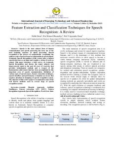
Figure 1: Local displacement algorithm. The local displacement algorithm (LDA) works evaluating for each point in P its distance from the line segment that joins the previous and next point. More precisely, at the first (1) step, the distance di = dist(Pi , Pi−1 Pi+1 ) is calculated for every Pi . This value represents the maximum displacement between the line Pi−1 Pi+1 and Pi−1 Pi+1 , i = 1, . . . , n − 1. During this step, the simplification is initialized with the computation of the cost of all possible point eliminations. The actual simplification is performed by minimizing the local error, therefore the point to be eliminated is the one causing the minimum line deviation. At the next step, and similarly for the subsequent, the distances will be updated only for the points involved in the last removal, that is, the previous and next point of the removed point. Therefore only two new distances will be computed. It follows that the method is based on a sequence of local updates where, at each iteration, the current data set is slightly modified and changes are limited to the part which surrounds the removed point. The shape is therefore preserved. The computational complexity is linear in the number of points n, since at the initialization step n distance computations are required while at each other step only two distances are updated. If the simplification is run without the aim of building a multi-resolution model of the line, the process may stop when a threshold distance is reached, that is, when all remaining points are above the given threshold distance. But, if we think of iteratively removing points until the line is simplified to the segment joining the first and last point, a more interesting formulation can be given in terms of data rearrangement. Indeed, the LDA as well as many other methods for line simplification, reduces the number of points by sorting data according to a simplification criterion, typically the error associated to the simplification technique. Indirectly, these methods induce a rearrangement of the original data into a new set which corresponds to the sequence of points ordered according to the error criterion. More precisely, given a chain of n points P, its rearrangement is defined by a permutation over the indices of P j : {0, . . . , n} �→ {0, . . . , n}. Let us also consider at each
be a function on an
: f (x, y, z) = 0}.
Given a plane π of equation ax+by +cz +d = 0, (a, b, c) �= 0, the scan line of Σ with respect to π is represented by the line, possibly empty, defined as L := Σ ∩ π =
f (x, y, z) = 0, ax + by + cz + d = 0.
Chosen a scan direction (a, b, c) �= 0 the sampling of the surface Σ is described by the set {Li }m i=1
with
Li := Σ ∩ πi ,
πi : ax + by + cz + di = 0, i = 1, . . . , m. Therefore, each scan line is described by a set of points P = {Pi }n i=0 , which locates the associated polygonal curve S(P0 , . . . , Pn ) obtained joining consecutive points with a line segment. The constraint for scan lines of being planar is not strict, in the sense that the results still hold if the curves are not planar, provided that they do not intersect each other.
307
(k)
(k)
simplification step k a vector (di )n is the i=0 , where di value of importance of Pj(i) in the current simplified line. Let us now describe the behavior of LDA using the rearrangement and the importance vector. At the first step, the importance vector and the permutation are initialized as follows. If the following minimization criteria is used (1)
dk =
min
i=1,...,n−1
Indicated with Sr := (P0 , P1 , . . . , Pn ) the input data set at the original resolution, we want to construct its lower resolution version Sr−1 with m points, m ≤ n. Therefore, in the simplification from Sr to Sr−1 , (n − m + 1) points will be omitted with an amount of lost detail Dr−1 that will be estimated using the reference distance d. If this procedure is applied recursively, we may express Sr through a hierarchical structure of lower resolution descriptions S0 , . . . , Sr and of details D0 , . . . , Dr−1 as described in (2). Since Sr can be reconstructed from the sequence S0 , D0 , . . . , Dr−1 the process is a filter bank and it represents a hierarchical transformation of the sampled data set. Having introduced the outline of the multi-resolution analysis, we have to specify [11]:
(1)
{di }
then, the first values of the permutation j are j(0) = 0, j(1) = n, j(2) = k while the importance vector gets d0 = (1) (1) d1 = 0, d2 = dk . At the second step the array (di )n i=0 is updated with
• the simplification error between Sr and a lower resolution Sk ,
(1)
(2) di
=
di if i ∈ / {k − 1, k, k + 1} if i = k − 1 dist(Pk−1 , Pk−2 , Pk+1 ) dist(Pk+1 , Pk−1 , Pk+2 ) if i = k + 1.
(1)
• the expression of Sr using S0 , D0 , . . . , Dr−1 .
where dist is the Euclidean distance function between a point and a segment (see Figure 1), i.e. the cost function of the algorithm. Therefore, the cost function is recomputed only on the points Pk−1 , Pk+1 whose neighborhoods were affected by the elimination of Pk . After this update, the minimization criterion is applied and j(3) and d3 are defined. After (n − 1) steps the input polygonal line will be fully reordered by the complete permutation j : {0, . . . , n} �→ {0, . . . , n} together with the associated importance array (di )n i=0 . The simplification process could be biased by the presence of spikes in the scan line. Spikes are characterized by a sharp local variation of the scan line shape, and therefore they can be easily identified and removed before applying the LDA [9]. If spikes are not removed by a pre-processing, they could be retained in the simplified line. Conversely, small undulations are automatically corrected by the LDA simplification.
To formalize the error, let us introduce a sequence of strictly decreasing real non-negative error bounds, called α−set, {t1 , . . . , tr : t1 > . . . > tr , r ≥ 1} and let us define: • Sk the data set obtained from Sk+1 considering those points which fulfill the inequality d(Sk , Sk+1 ) ≤ tk+1 , • Dk := Sk+1 − Sk (note that Dk ∩ Sk = ∅, Sk+1 = Sk ∪ Dk ) ∀k = 0, . . . , r − 1 the data set of detail. From the previous relations, we have that Sk ⊆ Sk+1 and we can construct the sequence S0 ⊆ S1 ⊆ . . . ⊆ Sr and its filter bank Sr −→ Sr−1 −→
Dr−1
2.2 Multi-resolution model
... ...
−→ S1 −→ S0
D0
(2)
with
In this section we describe the multi-resolution representation of the input line data, independently of the chosen simplification criterion. In general, given a set P := {Pi }n i=0 , a simplification algorithm defines a new set Q = {Qi }m i=0 such that:
Sk = {Pj(i) ∈ Sk+1 : di ≥ tk+1 } = {Pj(i) ∈ Sr : di ≥ tk+1 } and Dk = {Pj(i) ∈ Sr : di < tk+1 }.
• Q is a subset of P (m ≤ n), • S(Q0 , . . . , Qm ) is a good approximation of S(P0 , . . . , Pn ), that is, the distance between P and the simplified line is less than a maximum tolerance with respect to a distance function d associated to the application context. Typically, d represents the Hausdorff or the Euclidean distance. As previously described, several methods for line simplification reduce the number of points by sorting data according to a simplification criterion, which induces a rearrangement of the original data into a new set. The new set corresponds to the sequence of points ordered according to the error criterion. The simplification process can be also expressed as the process of constructing lower resolution representations of the original line, therefore resulting in a sequence of lines at different levels of detail.
Therefore, Sk is obtained applying the algorithm with tk+1 either to Sr or to Sk+1 . The previous relations can be summarized as Sr = ∪r−1 k=0 Dk ∪ S0 that is, the original data set is uniquely decomposed using the low resolution description S0 and the detail sets (Dk )r−1 k=0 . To conclude, let us note that the multi-resolution scheme is general since it is described independently of the specific simplification used. The specific method used in combination with the proposed multi-resolution framework is described in the following section.
3. CLASSIFICATION PHASE The goal of the classification phase is to characterize the input data using a family of algorithms each one is related to a specific aspect of representation, more precisely the scale
308
• α-value similarity: P ∈ LP , Q ∈ LQ
(see Section 3.1) and the geometry (see Section 3.2). According to [4], we want to identify in the mathematical description of the object both a general aspect (i.e. its geometrical model) and a set of specific aspects induced by the application context. The mathematical description is defined by the notion of equivalence class. The idea is to translate the geometric information into mathematical relations and to use the classes induced in the quotient space to collect points with equal properties into non-empty, disjoint subsets. This approach represents an initial and general step for the identification of feature lines and the segmentation phase. Given a set X and a relation R on X, i.e. R is a subset of X × X, we can define, for every point x ∈ X, its equivalence class [x] as the set of points in X which are in relation with x, that is,
P ∼α Q ⇐⇒ dP , dQ belong to the same sub-interval of I where dK is the α-value that characterizes the point K in its scan line LK . Therefore, the multi-resolution model defines the relation ∼α which introduces a hierarchy of importance between the size of shapes related to each point in the input data set. Using the α-value criterion we are able to distinguish between local information and characteristic points which locate the line features of the object to be extracted in the next phase (see Section 4). More precisely, small undulations are located by points whose α-value belongs to the first subinterval I1 := (0, tr ] of I (i.e. detail points). Points belonging to other intervals are called characteristic or structural points.
[x] := {y ∈ X : xRy} ⊆ X,
3.2 Form feature similarity
and the quotient space X/R := {[x] : x ∈ X}. Furthermore, the following conditions hold:
The next classification phase is aimed to capture the geometry of shape features in the scan lines. Here, we have tried to use shapes which have a meaning in the machining context, such as slots, pockets or steps. The configurations shown in Figure 2 correspond to their shape as if they were digitized on the object. Input points are classified using their local behavior with respect to their neighbors on the line, and each point belongs to a unique type of geometric shape. Clearly, Figure 2 could be improved and tuned to the specific application domain, for example geographical information systems [11] or more general pattern recognition processes.
• [x] �= ∅, ∀x ∈ X (i.e. every class is not empty), • [x] ∩ [y] = ∅ iff (x, y) ∈ / R (i.e. two classes are disjoint if and only if their representative elements are not in relation), • X=
x∈X [x]
(i.e. {[x]}x∈X represents a cover of X).
Therefore, a symmetric, reflexive and transitive relation on a set X induces a decomposition into a family of non-empty, disjoint sets each one identifies all points in X which fulfills the ”property” described by R.
3.1 Scale analysis and α-value similarity The multi-resolution simplification provides the classification of scan line points with respect to different levels of detail (scale). In order to define an automatic and global characterization, the α-value di associated to each scan line is normalized in I := [0, 1] dividing it by the maximum value which has been stored during the re-ordering of the entire input data set. Considering a partitioning of I into r subintervals {(ti , ti+1 ]}ri=1 , t1 = 1, tr+1 = 0,
r
(ti , ti+1 ] = [0, 1) i=1
we apply the multi-resolution model using the α-set {1 = t1 , t2 , . . . , tr+1 = 0} and classifying each point with respect to its α-value which represents the scale of the shape it introduces on the line. Therefore, the most important vertices with respect to scale will be represented, for each polygonal line, by the set Q := {Pj(i) }n−1 i=i0 ∪ {P0 } ∪ {Pn } with i0 such that di0 > tr and di0 −1 ≤ tr . We underline that if the input data set is equally sampled the partitioning of I can be defined using a uniform distribution, that is r+1−i ti := r
Figure 2: Basic shape types: for each configuration, black dot represents that point at which the label is attached. Starting from this table, we define the following relation: • feature similarity: P ∈ LP , Q ∈ LQ P ∼T Q ⇐⇒ T (P ) = T (Q) where T (K) represents the class of K according to the basic shapes represented in Figure 2.
i = 1, . . . , r + 1
achieving good results without user interaction. In presence of unbalanced density and dimension of shape features a redistribution of the partitioning is applied taking into account prior information. Using the α−set, we introduce the following relation:
The feature similarity classification (see Section 5) is applied to each simplified polygonal line represented by characteristic points; in this way, we get rid of local perturbations in the data and we may use a global view of the shape.
309
4.
FEATURE LINE DETECTION
The importance of feature lines for reverse engineering has been stressed in [6, 21] even if knowledge of the morphological structure of a surface is important in many other contexts such as GIS [4] and computer vision [19]. The reconstruction of surface features relies on the assumption that the shape of adjacent profiles is similar for sufficiently dense data sets, i.e. the object surface varies with continuity. The background for the reconstruction is the analysis of each scan profile by using the previous classification. The extraction of feature lines across scan lines is achieved by considering the reciprocal position of characteristic points. More precisely, if p and q belong to adjacent scan lines, the point p will be linked to q if and only if their distance is less or equal to a given threshold η, i.e. �p − q� ≤ η (see Figure 3). This parameter represents the scan step used for the acquisition process; its role is to control the joining process whose reliability decreases when distance between points increases. In Figure 4, an example of characteristic points is presented.
(a)
(b)
(c)
(d)
Figure 5: (a) Input object with 19.967 points structured in 102 scan lines, (b) feature points, (c), (d) optimized feature lines. in a simple and efficient way, we enable the possibility of eliminating small branches. Given the penalty function F (L) :=
1 n
n−1
�Pi+1 − Pi �2 ,
(3)
i=0
where (Pi )n i=0 is a set of ordered points, and indicated with L1 and L2 the two feature lines which intersect in a common point P we will eliminate the polygonal line segment L1 which fulfills the condition
Figure 3: Example of construction of feature lines and splitting points. The point P is not connected to Q because �P − Q�2 > η.
|F (L1 ) − F (L2 )| ≤ �
(a)
where the threshold � is chosen by the user. An example of the result achieved by applying this criterion is shown in Figure 5. Furthermore, an overlapping test is performed in order to discover possible intersections between feature lines. Clearly, different changes to (3) are possible considering the application environment, the smoothness of the input data set and introducing weights for each line segment Pi Pi+1 , i = 0, . . . , n − 1. Another problem is represented by the scan direction, which is fundamental because feature lines whose direction is almost parallel to the scan direction will be difficult to detect. Therefore, this method recognizes feature lines in a direction almost orthogonal to the scan one by linking similar points from a line to the next one. This problem is not really critical for curved features; as shown in Figure 4 and 5, the main lines are successfully detected. Problems arise when the feature lines are completely orthogonal to the scan direction. Finally, since the feature extraction is done on the set of characteristic points only, the complexity of the extraction is obviously very attractive and the set of feature extracted,
(b)
Figure 4: Input object with 17.374 points structured in 99 scan lines, (b) characteristic points. A crucial part of the detection process is the selection of similar points because there may be a considerable number of candidates as well as none. In general, a point can be connected to one or more vertices, which belong to the same scan line, giving rise to a split of the feature line into two or more parts (see Figure 3). To handle this situation
310
even if not complete, may represent a very rich basis to perform a full segmentation of the data.
5.
SEGMENTATION
The focus of this section is on segmentation with the goal of subdividing the input data set into high-level features represented by closed regions with specific properties. Therefore, we want to define an hybrid method using a dedicated approach. Our approach to segmentation is based on the following definition given in [5]. Definition. 2. Let D represent the input data set (”entire image region”). Segmentation is the process that partitions D into n subregions R1 , . . . , Rn such that: 1.
n i=1
Figure 7: Segmentation.
Ri = D,
2. Ri is a connected region, i = 1, . . . , n, 3. Ri ∩ Rj = ∅, i �= j, 4. P red(Ri ) = TRUE, 5. P red(Ri ∩ Rj ) = FALSE, i �= j, (a)
where P red is a logical predicate on the points in D.
(b)
(c)
Figure 8: (a) Input object with 24.147 points structured in 139 scan lines, (b), (c) feature lines.
6. DISCUSSION AND FUTURE WORK The proposed model introduces a framework which enables a high-level description of densely sampled objects at different levels of detail. It represents the base of a structured approach to shape analysis and feature line extraction concerning reverse engineering of shape. In this sense, the use of the multi-resolution simplification aims at defining a hierarchical classification of points identifying structural parts in the input object. Finally, the feature line extraction and the segmentation of the input data set into non-empty, disjoint subsets have been defined exploiting the properties of the equivalence relations and of the induced quotient space. Our model can be extended to a triangular mesh converting its description to a set of scan lines achieved by the surface with a family of cutting planes. Because the proposed model only exploits the basic features preserved by the simplification phase it results independent from uniformity hypothesis on the object surface. Clearly, high-detailed data sets ensure better results especially in the feature line extraction reducing the number of disjoint arcs. Furthermore, it is possible to improve the quality of the feature line detection and segmentation using a supervising of the result with a subset of intervals in the partitioning of I or a part of the feature type classification in order to discard object features not meaningful with respect to the final result. The method is semi-automatic; user interaction is restricted to the choice of the parameters η and � which respectively control the feature extraction and its optimization. The parameter η is chosen as the average distance between consecutive scan lines and � is selected proportional to η. The proper setting of these parameters is strictly related to the quality of the measured data in terms of density and noise presence. Even if all presented tests have been obtained
Figure 6: Segmentation strategy. The segmentation is structured into two steps using the feature type similarity and a grouping process. In the first phase, the structural points, which define the global shape of the object surface, are classified using the feature similarity. In the second phase, each detail point p, which falls between two consecutive structural points v and w, is classified as its nearest one with respect to the medium point m which joins v and w (see Figure 6). This reflects the idea of transition from a shape to another; however, an unsolved problem is represented by the identification, in each scan line, of a region which locates this (shape) transition. The segmentation is induced by the predicate P red :=∼α ∩β where ∩ is the intersection of two relations and β is defined as follows: pβq if and only if p, q belong to a shape feature of the same type (with respect to the classification given in Figure 2) identified by 3 or 4 characteristic points in LP , LQ . The segmentation is visualized using colors identifying global areas of interest in the manufacturing context. In Figure 7, the segmentation has been applied to a metal mould.
311
using the previous criterion for selecting the thresholds, irregular objects require an interactive supervision in order to achieve meaningful results. In Figure 8, 9 feature lines have been successfully extracted even if small branches have not been removed by the optimization phase. The principal improvements of the described framework are intended to define a simplification algorithm fully integrated in the feature line extraction in order to minimize the number of disjoint arcs and to detect nested form features. The achievement of this result may allow to optimize the segmentation process producing more uniform regions in the input data set. Finally, a segmentation defined starting from feature lines is currently being studied.
[7]
[8]
[9]
[10] [11]
[12]
[13] (a)
(b)
(c)
Figure 9: (a) Input object with 16.883 points structured in 100 scan lines, (b) characteristic points, (c) segmentation.
7.
[14]
ACKNOWLEDGEMENTS
This work has been supported by the Project ”Sviluppo di Tecnologie Innovative per il Reverse Engineering e il Rapid Prototyping ed Analisi Comparative”, and the Bilateral Research Agreement ”Surfaces Segmentation and form feature identification” between IMA-CNR and Laboratory 3S, Ecole Nationale Sup´erieure d’Hydraulique et de M´ecanique, Grenoble. Thanks are given to the Computer Graphics Group of IMATI-GE and to B. Falcidieno and C. Pizzi.
8.
[15]
[16]
[17]
REFERENCES
[1] F. J. Canny. A computational approach to edge detection. IEEE Trans PAMI, 8(6):679–698, 1986. [2] P. Cignoni, C. Montani, and R. Scopigno. A comparison of mesh simplification algorithms. Computers and Graphics, 22(1):37–54, 1998. [3] D. H. Douglas and T. K. Peuker. Algorithms for the reduction of the number of points required to represent a line or its caricature. The Canadian Cartographer, 10(2):112–122, 1973. [4] B. Falcidieno and M. Spagnuolo. Shape abstraction tools for modeling complex objects. In Proceedings of the 1997 International Conference on Shape Modeling and Application (SMI-97), pages 16–25, Los Alamitos, CA, Mar. 3–6 1997. IEEE Computer Society. [5] R. C. Gonzales and R. E. Woods. Digital Image Processing. Addison-Wesley Publishing Company, 1993. [6] J. Hoschek, U. Dietz, and W. Wilke. A geometric concept of reverse engineering of shape:
[18]
[19] [20]
[21]
[22]
312
approximation and feature lines. In Mathematical methods for curves and surfaces II, pages 253–262, Nashville, 1998. In: M. Daehlen, Lyche T. and Schumaker LL. (eds), Vanderbilt University Press. A. Hubeli and M. Gross. Multiresolution feature extraction from unstructured meshes. In Proceedings of the Visualization 2001, pages 16–25, San Diego, CA, USA, 2001. IEEE Computer Society. J. Illingworth and J. Kittler. A survey of the Hough transform. Computer Vision, Graphics, and Image Processing, 44(1):87–116, Oct. 1988. X. Y. Jiang and H. Bunke. Fast segmentation of range images into planar regions by scan line grouping. Technical Report IAM 92-006, 1992, April. M. Kass, A. Witkin, and D. Terzopoulos. Snakes: Active Contour Models . Academic Publishers, 1987. G. Patan´e and M. Spagnuolo. Scale-based segmentation of digitized data. Report 10/2001, Istituto per la Matematica Applicata, Consiglio Nazionale delle Ricerche, October 2001. A. Raviola, M. Spagnuolo, and G. Patan´e. Feature lines reconstruction for reverse engineering. Lecture Notes in Computer Science, 2181:18–30, 2001. C. Rossl, L. Kobbelt, and H. Seidel. Extraction of feature lines on triangulated surfaces using morphological operators. In Smart Graphics 2000. AAAI Spring Symposium, Stanford University, 2000. R. Sacchi, P. J.F., P. Thomas, and K. Hafele. Curvature estimation for segmentation of triangulated surfaces. In Proceedings of 2nd International Conference on 3-D Digital Imaging and Modelling, pages 536–544, Ottawa, Canada, October 1999. 3DIM’99. E. Saux and M. Daniel. Data reduction of polygonal curves using b-splines. In Computer Aided Design, pages 507–515. Elsevier, October 1999. W. Schroeder. Polygon reduction techniques. In ACM Com. Graph. Proc. Annual Conf. Series Siggraph ’95, pages 1.1–1.14. Course Notes 30, October 1995. Y. Shinagawa, T. Kunii, A. Belayev, and T. T. Shape modeling and shape analysis based on singularities. International Journal of Shape Modeling, 2(1):85–102, 1996. E. J. Stollnitz, T. D. DeRose, and D. H. Salesin. Wavelets for computer graphics: a primer, part 1. IEEE Computer Graphics and Applications, 15(3):76–84, May 1995. E. Trucco and A. Verri. Introductory to techniques for 3-D computer vision. Prentice Hall, 1998. T. Varaday, P. Benk¨ o, and G. Kos. Reverse engineering regular objects: simple segmentation and surface fitting procedures. International Journal of Shape Modeling, 4(34):127–140, 1998. T. V´ arady, R. R. Martin, and J. Cox. Reverse engineering of geometric models - an introduction. Computer-Aided Design, 29(4):255–268, 1997. D. J. Williams and S. Mubarak. A fast algorithm for active contours and curvature estimation. Computer Vision, Graphics, and Image Processing. Image Understanding, 55(1):14–26, Jan. 1992.