Multi-Response Simulation Optimization Using Genetic Algorithm Within Desirability Function Framework Seyed Hamid Reza Pasandideh, Ph.D. Candidate Department of Industrial Engineering, Sharif University of Technology P.O. Box 11365-9414 Azadi Ave., Tehran, Iran Phone: +98 912 1721820, Fax: +98 21 6005116, E-mail:
[email protected]
Seyed Taghi Akhavan Niaki, Professor Department of Industrial Engineering, Sharif University of Technology Phone: +98 21 6165740, Fax: +98 21 6005116, E-mail:
[email protected]
Abstract This paper presents a new methodology to solve multi-response statistical optimization problems. This methodology integrates desirability function and simulation approach with a genetic algorithm. The desirability function is responsible for modeling the multi-response statistical problem, the simulation approach generates required input data from a simulated system, and finally the genetic algorithm tries to optimize the model. This methodology includes two methods. The methods differ from each other in controlling the randomness of the problem. In the first method, replications control this randomness and, while in the second method we control the variation by statistical tests.
Key Words: Multi-Response, Genetic Algorithm, Desirability Function, Simulation.
1. Introduction and Literature Review
1
A usual problem in the real world environment involves selecting a set of input conditions (the x’s being independent variables) which will result in a product with a desirable set of outputs (the y’s being response variables). Essentially, this becomes a problem in the simultaneous optimization of the response variables, each of which depends upon a set of independent variables x1 ,..., x p . In this problem, we wish to
select the levels of the independent variables such that all the response variables optimize. In this case, however, the selected levels of the x’s that optimize for example y1 might not even come close to optimize y2 . As an example, in quality control environments the goal may be to find the levels of the input variables (quality characteristics) of the process so that the quality of the product or responses has the desired characteristics. Also, in Response Surface Methodology (RSM) [23] we adjust the levels of the input variables until the set of outputs are optimized. In most RSM problems, the form of relationship between the response and the independent variables is unknown. Thus, the first step in RSM is to find a suitable approximation. Usually, a low-order polynomial is employed. If there is curvature in the system, then a polynomial of higher degree, mainly second order is used. Then, by a sequential procedure and the method of steepest ascent or steepest descent the best set of input for response is determined. RSM usually works well when we consider one response. Also, we usually do not apply RSM in complex cases such as non-polynomial and higher-order or multi–modal functions. While many real world problems involve analysis of more than one response variable, most of the mathematical programming applications in the literature have been focusing on single response problems and few attempts have been made to solve multiple-objective statistical problems. We can classify these attempts into four categories [2,10]. The usual practice in the first category is to simplify the problem, selecting the most important response and ignoring the other responses or considering them as the model constraints. For example, we can refer to Hartmann & Beaumont [18] and Biles [4]. While Hartmann & Beaumont modeled the problem using linear programming approach, Biles used this approach once in conjunction with a version of Box’s complex method [7] and alternatively along with a variation of the gradient method. The proposed procedures of this category would generally lead to unrealistic solutions, especially when conflicting objectives are present. For example, in a capital investment problem with two objectives, profit maximization and risk minimization, it usually happens that the higher the profit the bigger the risk. For this reason, treating this problem using a single objective will lead to a poor solution. In the second category, in which we basically aggregate the objectives into a single objective function, has been attempted several times in the literature, each time with relative successes [10]. One of these attempts is called the weighted sum method and consists of adding all the objectives together using different weighting coefficients. Also a variation of the goal programming methods falls in this category. For instance, Clayton et al. [9], Rees et al. [25] and Baesler & Sepulveda [3] used this approach along with other optimization methods. Baesler & Sepulveda integrated the goal programming and genetic algorithm (GA) methods to solve the problem. Moreover,
2
they used some statistical tests to control the random nature of the problem. Another method in this category is the goal attainment method in which in addition to the goal vector for each response, a vector of weights relating the relative under or over attainment of the desired goals must be elicited from the decision maker. The most serious pitfall of the methods in this category is the importance of the responses and hence the determination of the weights in the objective function In the third category, some multi-attribute value functions are used. Mollaghasemi et al. [21] used a multi-attribute value function representing the decision-maker preferences. Then, they applied a gradient search technique to find the optimum value of the assessed function. Moreover, Mollaghasemi & Evans [22] proposed a modification of the multi–criteria mathematical programming technique called STEP method which works in interaction with the decision-maker. Teleb & Azadivar [27] proposed an algorithm based on the constrained scalar simplex search method. This method works by calculating the objective function value in a set of vertices of a complex. It moves towards the optimum by eliminating the worst solution and replacing it with a new and better solution. The process repeats until a convergence criterion is met. Boyle [6] presented a method called Pair-wise Comparison Stochastic Cutting Plane (PCSCP) which combines features from interactive multi-objective mathematical programming and response surface methodology. In the fourth category, a search-heuristic algorithm is basically used. Cheng et al. [8] presented a neuro-fuzzy and GA method for optimizing the multiple response problems. Schaffer [26] introduced a new method, called the vector evaluated genetic algorithm (VEGA), which differed from the simple GA method in the way of the chromosomes selection. Allenson [1] used a population–based modeling on VEGA, in which gender was used to distinguish between the two objectives of a problem consisting of planning a route composed of a number of straight pipeline segments. In this method only male-female mating is allowed and gender is randomly assigned at birth. Fourman [15] suggested a GA based method on lexicographic ordering problem. In his approach, the designer ranks the objectives in order of importance. The optimum solution is then obtained by optimizing the objective function, starting with the most important and proceeding according to the assigned order of importance. Periaux et al. [24] proposed a GA-based method that uses the concept of game theory to solve a bi-objective optimization problem. Coello [11] proposed minmax strategy with GA. In his method, the decision maker has to provide a predefined set of weights that will be used to spawn several small subpopulations that evolve separately, each trying to converge to a single point. Fonseca and Fleming [14] proposed a GA scheme in which the rank of an individual corresponds to the number of chromosomes in the current population by which it is dominated. Kim and Rhee [20] proposed a method based on the desirability function and GA and applied his method to optimize a welding process. Heredia-Langner et al. [19] presented a modelroboust alphabetically-optimal design with GA. This technique is useful in situations when computer-generated designs are most likely to be employed. In summary, the review of the literature in this category reveals that the Genetic Algorithm (GA) method has a specific role and works successfully.
3
In section two, we will give a brief description of the desirability function approach. Then, we model a multi-response statistical optimization problem through the desirability function method in section three. In section four, we will present two procedures, both based on the GA approach, to solve the problem. In order to evaluate the performance of the proposed procedures and to compare them, we will solve some numerical examples and will report the results in section five. Finally, in section six we will have the conclusion and some recommendations for future research.
2. Desirability Function The desirability function approach is one of the most widely used methods in industry for dealing with the optimization of multiple-response problems. It is based on the idea that the quality of a product that has multiple quality characteristics is completely unacceptable if one of the characteristics lies outside the desired limits. This method assigns a score to a set of responses and chooses factor settings that maximize that score. In order to describe the desirability function approach mathematically, suppose each of the k response variables are related to p independent variables by equation (1).
y ij = f i ( x1 ,..., x p ) + ε ij
i =1,..., k , j =1,.., ni
(1)
where y ij is the jth observation on the ith response and f i denotes the relationship between the ith response, y i , and x1 , ..., x p .The parameter ni is the maximum number of observations for each of the k responses and ε ij is an error term with mean E (ε ij ) = 0 and variance VAR (ε ij ) = σ i such that we can relate the average response to the p independent variables by equation (2). 2
η i = f i ( x1 , ..., x p )
i = 1,..., k
(2)
A desirability function, d i ( yi ) , assigns numbers between 0 and 1 to the possible value of each response y i . The value of d i ( yi ) increases as the desirability of the corresponding response increases. We define the overall desirability, D, by the geometric mean of the individual desirability values shown in equation (3). 1
D = (d 1 ( y1 ) × d 2 ( y 2 ) × ... × d k ( y k ) ) k
(3)
where k denotes the number of the responses. Note that if a response y i is completely undesirable, i.e., d i ( yi ) =0, then the overall desirability value is zero.
4
Depending on whether a particular response y i is to be maximized, minimized, or assigned a target value, we can use different desirability functions. Derringer & Suich [13] introduced a useful class of desirability functions. There are two types of transformation from y i to d i ( yi ) , namely one-sided and twosided transformation. We employ the one-sided transformation when y i is to be maximized or minimized, and the two-sided transformation when y i is to be assigned a target value. In a two-sided transformation assume li and u i be the lower and upper limits and ti be the target value of the response y i respectively such that l i < t i < u i . Then we define the desirability function as equation (4). yi < li
0,
(
di ( yi ) =
yi − li s ) , t i − li
li ≤ yi ≤ t i
yi − ui t ), ti − ui
ti ≤ yi ≤ ui
0,
yi > ui
(
(4)
where the exponents s and t determine how strictly target value is desired and the user must specify their values. For s=t=1 the desirability function increases linearly towards ti, for s1 the function is concave. This function for different values of s and t is graphed in Figure (1).
1
Desirability
s=0.5
t=0.5
0.5 t=1 Figure (1).s=1 Graph of the two-sided transformation s=5
t=5
0 Response
In Figure (1) we choose the value of ti to be in the almost lower 25% of the interval between li and ui. From Figure (1) we can see that the large values of s and t are 5
chosen for situations in which we need to have the response near ti. In situations in which we desire to have the response near li we choose the values of t and s small. We use medium values for s and t (close to one) when a case between the above two extremes is desired. Furthermore, if the user wants to have the response get closer to ti very fast and any value for the response greater than ti and less than ui is desirable, then he chooses the value of s to be large and the value of t to be small. Similarly, we can define one-sided desirability functions for minimizing or maximizing case. It should be noted that while some modified versions of the desirability functions are useful for situations in which the exact mathematical methods of optimization is used, the introduced basic desirability functions is good enough for the search methods applied for optimization problems [12]. For a good reference, see Derringer and Suich [13].
3. Problem Modeling The candidate problems in the framework of this research have two main characteristics. First, the problem itself is a computer simulation of a real world problem. For example, we simulate a real world production system in which events occur stochastically and there are different factors affecting multiple responses simultaneously and the goal is to determine the levels of the factors that optimize the responses. In this case, when we select different inputs as the levels of the factors, the values of the responses are observed by simulation. Second, the levels of the factors can be modeled by a real variable. A real example to the problems having these characteristics is a quality control process in which the reaction time, the temperature and the percent catalyst are the input variables and the responses are the percent conversion and thermal activity of the process. In this situation we may first want to simulate the production process and then we want to determine the input variable levels such that the outputs maximized or minimized or set to a target value. In the modeling phase of a multi-response statistical optimization problem, we transform the objective function to a single function using the desirability function framework. First we identify: 1. All the factors that make up the input of the problem. These factors are the independent variables x1 ,..., x p . 2. The lower and upper bounds of the independent variables ( L ( x h ) and
U ( x h ) ). 3. The output of the problem. This output is the response variables denoted by y1 ,..., y k . 4. One-sided or two-sided desirability functions for each response. It is obvious that a one-sided or two-sided transformation for each response depend on the nature of the objective of the problem. Then the mathematical model of the problem becomes:
6
max D = k (d 1 ( y 1 ) × d 2 ( y 2 ) × ...× d k ( y k )) s .t .:
(5)
L (x h ) ≤ x h ≤ U (x h ) h = 1, 2,..., p
In the next section we present two methods to solve model (5) based on the lowest error criterion.
4. The Methodology In order to solve model (5), first we employ a simulation approach to generate output response values for all the objectives in the problem. Note that the problem has a stochastic nature. This means if the set of x1 ,..., x p is fixed, then in each of the simulation execution case the set of y1 ,..., y k may be different. Because of the stochastic nature of the model, we need to apply a heuristic-search algorithm to solve it. Among these algorithms, GA is shown to be successful in optimizing the multi-response problems, especially when we combine the objectives into one objective [10]. The usual form of GA was described by Goldberg [17]. Genetic algorithms are stochastic search techniques based on the mechanism of natural selection and natural genetics. GA is differing from conventional search techniques in a sense that it starts with an initial set of random solutions called population. Each individual in the population is called a chromosome, representing a solution to the problem at hand. The chromosomes evolve through successive iterations, called generations. During each generation, the chromosomes are evaluated, using some measures of fitness. To create the next generation, new chromosomes, called offspring, are formed by either crossover operator or mutation operator. A new generation is formed according to the fitness values of chromosomes. After several generations, the algorithm converges to the best chromosome. Knowing that a GA method needs scalar fitness information to work, the simplest idea that we could devise is to combine all the responses into a single one. In this methodology, we use desirability approach for combining all the responses. Desirability functions have many advantages in comparison to other combining techniques, especially, they have very flexible role. It means we can simultaneously maximize some of responses and minimize others and setting target value to some of them.
4.1. Initial Conditions
7
The initial information required to start the GA methods follows: 1. Population size: It is the number of the chromosomes or scenarios that we will keep in each generation and we denote it by N. 2. Number of replications: It is the number of the simulation replications of each scenario and we denote it by n. 3. Crossover rate: This is probability of performing crossover in the GA methods, which is denoted by Pc . 4. Mutation rate: This is probability of performing mutation in the GA method denoted by PM . 4.2. Chromosome
In the GA methods, we define chromosomes or scenarios being a set of the values for x1 ,..., x p as a solution to the problem. 4.3. Initial Population
Generating an initial population of solutions or scenarios is the first stage to start the optimization process. The number of the scenarios is N and we select the scenarios randomly to cover a wide range of the solutions. Generally, users have a good idea where they can find good solutions. We can consider some of the user’s suggestions in the initial population. In order to obtain the total desirability value of scenario j, x1 j , x 2 j , ..., x pj , after its preparation, we simulate it in n replications. Then, in each replication, we generate the response variables and determine the desirability value of each response. To do this we define the following parameters: xij : Is the input variable i in scenario j, i =1,.., p , j =1,.., N . y ijr : Is the response variable i in scenario j and in replication r, i = 1,.., k , j = 1,.., N , r =1, ..., n . d ijr : Is the desirability i in scenario j and in replication r, i = 1,.., k , j = 1,.., N , r =1, ..., n and we obtain its value based on the desirability function characteristics described in section two. D jr : Is the total desirability value of scenario j in replication r, j =1,.., N , r =1, ..., n . D j : Is the mean of the total desirability in scenario j, j = 1,.., N and we calculate it by n
D j = ∑ D jr / n r =1
S j : Is the standard deviation of the total desirability in scenario j, j = 1,.., N .
4.4. Crossover and Mutation
8
In a crossover process, it is necessary to mate pairs of chromosomes to create offspring. We perform this by selecting a pair of chromosomes from the generation randomly and with probability Pc . There are many different types of crossover operators. In this research, we use a variation of the crossover operators that work very well when the chromosome is represented using real code and not binary code [16]. To define this operator precisely, assume that chromosomes A and B, presented respectively in the forms [a1 , a2 , ..., a p ] , [b1 , b2 , ... , b p ] , are selected for the crossover operation. This crossover operator by the following relations will create the new chromosomes C and D: (6) C = λA + (1 − λ ) B D = (1 − λ ) A + λB (7) where λ is a parameter ranging between 0 and 1. One of the advantages of this crossover operator is that the new chromosomes C, D will be feasible. Mutation is the second operation in the GA methods for exploring new solutions. In mutation, we replace a gene with a randomly selected number within the boundaries of the parameter [16]. More precisely, assume a specific gene such as a j is selected for mutation, then we change the value of a j to the new value a *j according to equations (8) and (9), randomly and with the same probability: i ) max gen i a*j = a j − ( a j − l j ) × r ×( 1 − ) max gen
a *j = a j + ( u j − a j ) × r × ( 1 −
(8) (9)
where l j and u j are the lower and upper limits of the specified gene, r is a uniform random variable between 0 and 1, i is the number of current generation, and maxgen is the maximum number of generations. Note that the value of a j is transferred to its right or left randomly by equations (8) and (9) respectively and r is this percentage. Furthermore, 1 −
i max gen
is an index with a value close to one in the first generation
and close to zero in the last generation that makes large mutations in the early generations and almost no mutation in the last generations.
4.5. Objective Function Evaluation
After producing the new chromosomes by crossover and mutation processes, we must simulate them. We can generate the value of response variables, desirability functions and total desirability for each of the new scenarios by simulation. 4.6. Chromosomes Selection
9
In the next phase of the methodology, we select the chromosomes for the next generation. This selection is based on the fitness function value of each chromosome. The difference of the two proposed GA methods appears in this phase. In the first method, we consider the fitness function being the total desirability, D j , of scenario j and based on the better value of D j we select N chromosomes among the old and new ones deterministically. However, in the second method, we select the chromosomes statistically. In this regard, first we statistically compare the D j s and then select the ones with better values. To do this we apply two different multiple-comparison statistical tests [23] to control the random nature of the situation and group chromosomes such that there is no statistical difference within the groups but there exist differences among different groups. The multiple-comparison test used in the second method is the Tukey’s test[23]. Tukey’s test determines a critical value, Tα , such that the probability of making a type Ι error is α for all comparisons. Any pairs of D j s that differ by less than Tα are statistically equal. The value of Tα is determined by equation (10). Tα = qα ( N , f ) ×
MSE
(10)
n
where qα ( N , f ) is the upper percentage point of the Studentized Range Statistic [16], N is the population size, MSE is the mean squared error of D j s, and f is the degrees of freedom associated with MSE which is equal to n(N-1). Now based on the fitness function value, we rank the chromosomes in ascending order and group them with a difference between their fitness function values less than Tα accordingly. In this way, we create groups of chromosomes that are not statistically different. In order to generate chromosomes for the next generation, we apply the roulettewheel-selection technique [5, 16], which is the most common selection technique. In this technique, first we calculate the probability of selecting group k, p k , by equation (11) as:
∑D
pk =
j
∀j ∈ Group k N
∑D
(11)
j
j =1
Then by the roulette-wheel-selection method, we choose a group randomly and select its best chromosome based on its fitness function value. We do this N times making a generation with N chromosomes. After we create the next generation, the crossover and mutation operators will operate on the new generation again and we will repeat the selection phase. This loop continues until the stopping criteria are met.
10
4.7. Stopping Criteria
The last step in the methodology is to check if the selected method has found a solution that is good enough to meet the user’s expectations. Stopping criteria is a set of conditions such that when the method satisfies them, a good solution is obtained. In this research, we stop when we observe no improvement in fitness function values of several consecutive generations. The number of sequential generations depends on the specified problem and the expectations of the user.
5. The Performance of the Proposed Methods Since most of the applications of the new methods are in the quality control and RSM environments and considering the fact that we use polynomials in these situations, in order to evaluate the performance of the new methods and to compare them, we apply different polynomial examples. The examples of the experiments are polynomial in nature such that when the values of the independent variables are fixed the expected values of the responses are known. For example, consider three responses (output variables) as polynomial functions of three independent variables (input variables) as: y1 = x15 + x14 + x 23 + x 36 + x1 x 2 x 3 + ε 1
y 2 = x12 + x1 x3 + x 2 x3 + x1 x 2 x3 + ε 2 y 3 = x13 + x 23 + x34 + x1 x 22 x34 + ε 3 where ε 1 , ε 2 , and ε 3 are the error terms with the following distributions; ε 1 ~ N [ 0 ,1] , ε 2 ~ EXP ( 0.10 ) , ε 3 ~ N [ 2,4] , and the input variables ranging in 0 ≤ x1 ≤ 5 , 0 ≤ x 2 ≤ 3 , and 0 ≤ x 3 ≤ 4 . Note that for a fixed values of the independent variables as x1 = 2 , x 2 = 1 , and x3 = 3 the average value of responses will be T1 = E ( y1 ) = 784 , T2 = E ( y 2 ) = 19.1 , and T3 = E ( y 3 ) = 254 . In this case, based on the fixed values of the response being T1=784, T2=19.1, and T3=253 and applying a two-sided desirability function described in section two, the method that reaches to these values of the independent variables closer has better performance than the other does. Thus, in order to compare the methods, we define a performance measure as: p
e2 ( m )=
∑ (x
j
( m ) − x j ( a )) 2
(12)
j =1
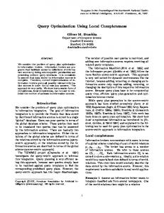
We apply both methods to the different examples, each time calculating the performance measure in equation (12).We employ five different polynomial functions in four types of replications, making the total number of examples 80. For all of the examples we apply a two-sided desirability function with the parameters s and t both being equal to one and the type I error in Tukey’s test being equal to 0.05. Moreover we generate the value of the responses in each method by random numbers
11
from error term 's polynomials. Figure (2) shows the results of performance measure versus to different replications.As we see, the first method is better than second method .
Error
1st method
2nd method
10 8 6 4 2 0 5
10
25
50
Replication
Figure (2).Graph of the performance
6. Conclusion and Recommendations for Future Research In this paper, we modeled a multi-response statistical optimization problem through the desirability function approach. Then we applied two GA methods to solve this model by simulation. We studied the performance of each method through different simulation replications. For future researches in this area, we recommend the followings: 1. In cases when the user has no idea about how to set the parameters l and u in the initial step, we can assign them their extreme values. Then we apply the method sequentially, selecting the best solution in each step. Next, we replace the solution with l in maximization case and with u in minimization environment. This process continues until we obtain no feasible solution. 2. In addition to the Tukey’s test, we can perform other multiple comparison tests. Then we can compare the performance of other statistical tests in this regard. 3. Different crossover and mutation operators in the GA methods may lead to different conclusions. 4. Instead of selecting the chromosomes based on their fitness function values, we can choose them randomly. This will lead us in another research when a comparison can be made between the two ways of chromosome selection. 5. Instead of preparing the data by simulation, the method can apply to real world situation, such as quality improvement in an industry, where we are to choose the best subset of the input variables for multi-response optimization purposes. 6. Rather than polynomials, we can evaluate the performance of the method by some other functions of the input variables. 7. A comprehensive set of benchmark cases is needed for the comparison purposes of the performance of different search-heuristic methodologies in this area.
7. References
12
1. 2. 3.
4. 5.
6. 7. 8.
9.
10. 11.
12.
13. 14.
15.
16. 17. 18.
Allenson, R. Genetic algorithms with gender for multi-function optimization. EPCC-SS92-01. University of Edinburgh, 1992. Azadivar, F. Simulation optimization methodologies. Proceedings of the 1999 winter simulation conference, 1999. Baseler, F. F., & J. A. Sepulveda. Multi-response simulation optimization using stochastic genetic search within a goal-programming framework. Proceedings of the 2000 winter simulation conference, 2000. Biles, W. E. & J. J. Swain. Optimization and Industrial experimentation. Wiley Inter-science, New York, 1980. Boesel, J., B. Nelson, & N. Ishii. A framework for simulation optimization software. Technical Report, Dept. of industrial Engineering and Management Sciences, Northwestern University, 1999. Boyle, C. R. An interactive multiple response simulation optimization method. IIE Transactions, 14, pp. 453-463, 1996. Box, G. E. P., & P. Y. T. Liu. Empirical model building and response surface. John Wiley & sons, New York, 1987. Cheng, B. C, C. J Cheng, & E. S. Lee. Neuro-fuzzy and genetic algorithm in multiple response optimization. Computers and mathematics with applications. 44, pp.1503-1514, 2002. Clayton, E. R., W. E. Weber, & B. W. Taylor. A goal programming approach to the optimization of multi-response simulation models. IIE Transactions, 14, pp. 282-287, 1982. Coello Coello, C. A. An updated survey of GA-Based multi-objective optimization techniques. ACM computing surveys, 32, pp.109-143, 2000. Coello Coello, C. A. An empirical study of evolutionary techniques for multiobjective optimization in engineering design. Ph.D. dissertation, Tulane University, 1996. Del Castillo, E., D. C. Montgomery & D. R. Mcarville. Modified desirability functions for multiple response optimizations. Journal of Quality Technology, 28, pp.337-345.1996. Derringer, G. & R. Suich. Simultaneous optimization of several response variables. Journal of Quality Technology, 12, pp. 214-219, 1980. Fonseca, C. M. & P. J. Fleming. Genetic algorithm for multi-objective optimization: formulation, discussion and generalization. Proceedings of the fifth international conference on genetic algorithms, pp.416-423, 1993. Fourman, M. P. Comparison of symbolic layout using genetic algorithms. Proceedings of the first international conference on genetic algorithms and their applications, pp.141-153, 1985. Gen, M. Genetic algorithm and engineering design, 1997. Goldberg, D. Genetic algorithms in search, optimization and machine learning, 1989. Hartmann, N. E. and R. A. Beaumont. Optimum compounding computer. Journal of the Institute of the rubber Industry, 2, pp. 272-275, 1968.
13
19. Heredia-Langner, A., D. C. Montgomery, W. M. Carlyle, & C. M. Borror. ModelRobust optimal designs: a genetic algorithm approach. Journal of Quality Technology. 36, 2004. 20. Kim, D. and S. Rhee. Optimization of a gas metal arc welding process using the desirability function and the genetic algorithm. Proceedings of the institution of mechanical engineers, part B: Journal of engineering manufacture, Vol. 218, No.1 ,pp.35-41, 2004. 21. Mollaghasemi, M., M. G. Evans, & W. E. Biles. An approach for optimizing multiple response simulation models. In proceedings of the 13th annual conference on computers in industrial engineering, pp. 201-203, 1991. 22. Mollaghasemi, M. and G. W. Evans. Multi-criteria design of manufacturing systems through simulation optimization. Transactions on systems, man, and cybernetics, 29, pp. 113-121, 1994. 23. Montgomery, D. C., Design and analysis of Experiments. Fourth edition, 1997. 24. Periaux, J., M. Sefrioui, & B. Mantel. GA multiple objective optimization strategies for electromagnetic backscattering. Engineering and computer science, pp.225-243.1996. 25. Rees, L. P., E. R. Clayton, & B. W. Taylor. Solving multiple response simulation optimization models using modified response surface methodology within a lexicographic goal-programming framework. IIE Transactions, 17, pp.447-457, 1985. 26. Schaffer, J. D., Multiple objective optimization with vector evaluated genetic algorithms. Proceedings of the first international conference on genetic algorithms and their applications, pp.93-100, 1985. 27. Teleb, R., & F. Azadivar. A methodology for solving multi-objective simulation optimization problems. European Journal of operational research.72, pp. 135-145, 1994.
14