Multi-user Linear Precoding for Multi-polarized Massive MIMO ... - Core

1

Multi-user Linear Precoding for Multi-polarized Massive MIMO System under Imperfect CSIT Jaehyun Park, Member, IEEE, Bruno Clerckx, Member, IEEE,

Abstract— The space limitation and the channel acquisition prevent Massive MIMO from being easily deployed in a practical setup. Motivated by current deployments of LTE-Advanced, the use of multi-polarized antenna elements can be an efficient solution to address the space constraint. Furthermore, the dualstructured precoding, in which a preprocessing based on the spatial correlation and a subsequent linear precoding based on the short-term channel state information at the transmitter (CSIT) are concatenated, can reduce the feedback overhead efficiently. By grouping and preprocessing spatially correlated mobile stations (MSs), the dimension of the precoding signal space is reduced and the corresponding short-term CSIT dimension is reduced. In this paper, to reduce the feedback overhead further, we propose a dual-structured multi-user linear precoding, in which the subgrouping method based on copolarization is additionally applied to the spatially grouped MSs in the preprocessing stage. Furthermore, under imperfect CSIT, the proposed scheme is asymptotically analyzed based on random matrix theory. By investigating the behavior of the asymptotic performance, we also propose a new dual-structured precoding in which the precoding mode is switched between two dualstructured precoding strategies with i) the preprocessing based only on the spatial correlation and ii) the preprocessing based on both the spatial correlation and polarization. Finally, we extend it to 3D dual-structured precoding. Index Terms— Multi-polarized Massive MIMO, Dual structured precoding with long-term/short-term CSIT

I. I NTRODUCTION By deploying a large number of antenna elements at the base station (BS), high spectral efficiencies can be achieved. Furthermore, because low-complexity linear precoding schemes can be efficiently exploited to serve multiple mobile stations (MSs) simultaneously, Massive MIMO plays a key role in beyond 4G cellular networks ( [1]–[4] and references therein). Assuming large scale arrays, several linear single-user and multi-user precoding schemes are asymptotically analyzed by using random matrix theory in [5]–[9]. In [5], singleuser beamforming in MISO with a large number of transmit antenna elements has been analyzed under the per-antenna constant-envelope constraints and its extension to multi-user MIMO is treated in [6]. In [7], by utilizing a Stieltjes transform of random positive semi-definite matrices, the asymptotic A part of this work was published in the 22nd European Signal Processing Conference EUSIPCO 2014. J. Park is with the Department of Electronic Engineering, Pukyong National University, Republic of Korea. B. Clerckx is with the Department of Electrical and Electronic Engineering, Imperial College London, United Kingdom and also with School of Electrical Engineering, Korea University (e-mail:[email protected], [email protected]). B. Clerckx is the corresponding author. This work is partially supported by Huawei Technologies Co., Ltd.

signal-to-interference-and-noise ratio (SINR) of linear precoding in a correlated Massive MISO broadcasting channel has been derived under imperfect channel state information at the transmitter (CSIT). In [9], by considering multi-cell downlink with massive transmit antenna elements, the asymptotic SINR is analyzed by using random matrix theory which gives an insight about the cooperative transmission strategy of BSs. However, in FDD, where channel reciprocity is not exploitable, the multi-antenna channel acquisition at the transmitter prevents Massive MIMO from being easily deployed. To resolve the channel acquisition burden at BS, a dual structured precoding, in which a preprocessing based on the long-term CSIT (mainly, spatial correlation) and a subsequent linear precoding based on the short-term CSIT (that generally has lower dimension than the number of transmit antenna elements) are concatenated, can be exploited to reduce the feedback overhead efficiently [8], [10]. Note that the longterm CSI is slowly-varying and can be obtained accurately with a low feedback overhead. Because of the low feedback overhead and the attractive performance, the dual structured precoding has been also considered in the 4G and beyond 4G wireless standards [10], [11]. In [8], when MSs are clustered as several spatially correlated groups, joint spatial division and multiplexing scheme has been proposed in which the precoding matrix is composed of the prebeamforming matrix based on the spatial correlation and the classical precoder based on short-term CSIT. Furthermore, its performance is asymptotically analyzed for a large number of transmit antenna elements. Another challenge of the Massive MIMO system is the antenna space limitation. An increasing number of antenna elements is difficult to be packed in a limited space and if it can be deployed, the high spatial correlation and the mutual coupling among the antennas elements may cause some system performance degradation, especially for a small numbers of active MSs [12], [13]. The multi-polarized antenna elements can be one solution to alleviate the space constraint [14], [15]. The multi-polarized antenna systems have been investigated under various communication scenarios including the picocell/microcell [16], indoor/outdoor [17], and the line of sight (LOS)/non LOS (NLOS) [15] environments. However, despite the importance of polarized antennas in practical deployments, the Massive MIMO system with multipolarized antenna elements has not been addressed so far together with the multi-user linear precoding. Note that due to space constraints, closely spaced dual-polarized antennas is considered as the first priority deployment scenario for MIMO in LTE-A and is therefore likely to remain so as the number

2

of antennas at the base station increases [10], [11], [18]. In this paper, we first model the Massive multi-user MIMO system, where the BS is equipped with a large number of multi-polarized antenna elements. For simplicity and practical issue of MS, we consider that MSs are equipped with a single single-polarized antenna element. We then present the dual structured precoding based on long-term/short-term CSIT. As done in the Massive MIMO system with a single-polarized antenna element [8], by grouping the spatially correlated MSs and multiplying the channel matrix of the grouped MSs with the same preprocessing matrix based on spatial correlation, the dimension of the precoding signal space is reduced and the corresponding short-term CSIT dimension can also be reduced from the Karhunen-Loeve transform [19]. Considering the multi-polarized Massive multi-user MIMO system for the first time, the contributions of this paper are listed below: •

•

•

•

•

To reduce the feedback overhead further, we first propose a dual structured linear precoding, in which the subgrouping method based on the polarization is additionally applied to the spatially grouped MSs in the preprocessing stage. That is, by subgrouping co-polarized MSs in each group, we let the MS report the CSI from the transmit antenna elements having the same polarization as its polarization. Then, the MS can further reduce the shortterm CSI feedback overhead, compared to the case with the conventional preprocessing based only on the spatial correlation. Under the imperfect CSIT, two different dual structured precodings with preprocessing of i) grouping based only on the spatial correlation (i.e., spatial grouping) and ii) subgrouping based on both the spatial correlation and polarization are asymptotically analyzed based on random matrix theory with a large dimension [7]. Because, in this paper, the polarized Massive MU-MIMO channel is considered, the asymptotic inter/intra interferences are evaluated over the polarization domain as well as the spatial domain, which addresses a more general (polarized) channel environment compared to [7], [8]. Accordingly, the asymptotic performance can be further analyzed in terms of both the polarization and the spatial correlation and therefore, we can understand the performance behavior of dual structured precoding with respect to the long-term CSIT. We then propose a new dual precoding method to switch the precoding mode between two dual structured precoding strategies relying on i) the spatial grouping only and ii) the subgrouping based on both the spatial correlation and polarization. Motivated by 3D beamforming [8], [20], we extend the design to the 3D dual structured precoding in which the spatial correlation depends on both azimuth and elevation angles. Finally, we also discuss how we can modify the proposed precoding mode switching scheme when the polarization at the BS and MS is mismatched (due to e.g. random MS orientation).

Note that, from the asymptotic results, we can find that even

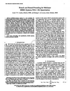
though the proposed dual precoding using the subgrouping can reduce the feedback overhead, its performance can be affected by the cross-polar discrimination (XPD) parameter. Here, XPD refers to the long-term statistics of the antenna elements and channel depolarization that measures the ability to distinguish the orthogonal polarization. That is, under the same feedback overhead, the dual precoding with subgrouping can utilize more accurate CSIT on half of the array, compared with precoding with spatial grouping, but exhibits performance more sensitive to the XPD. The precoding with spatial grouping can only utilize less accurate CSIT, but its performance is not affected by the XPD. Accordingly, we identify the region where the dual precoding with subgrouping outperforms that with spatial grouping. The region depends on the XPD, the spatial correlation, and the short-term CSIT quality, which motivated us to develop the new dual precoding method. The rest of this paper is organized as follows. In Section II, we introduce the Massive MIMO system model with multiple multi-polarized antenna elements at the BS and a (either vertically or horizontally) single polarized antenna element at the multiple MSs. In Section III, we discuss the dual structured precoding based on the long-term/short-term CSIT. In Section IV, we investigate the asymptotic performance of the dual precoding schemes and their behavior over the XPD parameter. Based on the asymptotic results, in Section V, we propose a new dual structured precoding/feedback. In Section VI, we provide several discussion and simulation results, respectively, and in Section VII we give our conclusions. Throughout the paper, matrices and vectors are represented by bold capital letters and bold lower-case letters, respectively. The notations (A)T , (A)H , (A)i , [A]i , tr(A), and det(A) denote the transpose, conjugate transpose, the ith row, the ith column, the trace, and the determinant of a matrix A, respectively. In addition, [A]i:j (resp., (A)i:j ) denotes the submatrix from the ith column (resp., row) to the jth column (resp., row) of A. The matrix norm ∥A∥ and the vector norm ∥a∥ denote the 2-norms of a matrix A and a vector a, respectively. In addition, A ≽ 0 means that a matrix A is positive semi-definite, ⊗ denotes the Kronecker product, and ⊙ denotes the Hadamard product. The operation Eg [Ag ] means the average of Ag over index g. Finally, IM , 1M ×N , and 0M ×N denote the M × M identity matrix, the M by N matrix with all 1 entries, and the M by N matrix with all 0 entries, respectively. II. S YSTEM MODEL We consider a single-cell downlink system with one BS with M polarized antenna elements and N active MSs, each with a single polarized antenna element, where M and N are assumed to be even numbers. As in Fig 1, the BS has M 2 pairs of co-located vertically/horizontally polarized antenna elements and the MSs have a single antenna element with either vertical or horizontal polarization1 . Furthermore, since 1 Throughout the paper, we consider the dual-polarized antenna elements at the BS for ease of explanation, but our approach can be extended to the tri-polarized case without difficulty. In addition, all the antenna elements are perfectly aligned with either vertical or horizontal polarization. In Section V-C, we discuss the polarization mismatch due to the random orientation of MSs.

3

magnitude. Note that generally, rg ≪ M , and Ug ∈ C 2 ×rg is composed of the eigenvectors of Rsg as its columns. The matrix Gg is defined as [ vv ] Gg Ghv g Gg = , (4) Gvh Ghh g g M

s1 D1

d1 MS group1

q1

BS q2

¯ N

rg × 2 , p, q ∈ {h, v} are i.i.d. and the elements of Gpq g ∈ C complex Gaussian distributed with zero mean and unit variance. The matrix X describes the power imbalance between the orthogonal polarizations and is given as [ √ ] 1 χ X= √ , (5) χ 1

MS group2

D2 Copolarized Subgroup

Fig. 1.

Block diagram of a dual-polarized multi-user downlink system.

human activity is usually confined in small clustered regions such as buildings, locations of MSs tend to be spatially clustered, e.g., G groups. Then, the received signal yg ∈ CNg of the gth group with an assumption of flat-fading channel is given by [ v ] yg = HH yg = (1) g x + ng , ygh where ygv and ygh are the received signal for MSs with ] [ vertical nvg is and horizontal polarization, respectively, and ng = nhg a zero-mean complex Gaussian noise vector having a covariance matrix INg , denoted as ng ∼ CN (0, INg ). Here, Ng denotes the number of MSs in the gth group. For simplicity, ¯ , where N ¯ is even, and it is assumed that N1 = ... = NG = N ¯ both ygv and ygh are N2 × 1 vectors. The channel of the kth MS in the gth group is then given as hgk = [Hg ]k . The M × 1 vector, x, is the linearly precoded transmit signal expressed as x=

G ∑ g=1

Vg dg ,

Vg ∈ CM ×N , ¯

(2)

] dvg are the linear precoding matrix dhg and the data symbol vector for the MSs in the gth group, respectively. The precoded signal x should satisfy the power constraint E[∥x∥2 ] ≤ P . [

where Vg and dg =

A. Channel model By using the Karhunen-Loeve transform [19] and the polarized MIMO channel modeling with infinitesimally small antenna elements described in [10], [14], the downlink channel to the gth group, Hg , can be represented as ([ )( ] ) 1 1 rxp Hg = Gg ⊙ (X ⊗ 1r× N¯ ) (3) ⊗(Ug Λg2 ) 2 rxp 1 where rxp is the correlation coefficient between vertically and horizontally polarized antenna elements, Λg is an rg × rg diagonal matrix with the non-zero eigenvalues of the spatial covariance matrix Rsg for the gth group2 , where the eigenvalues are assumed to be ordered in decreasing order of 2 For simplicity, it is assumed that the spatial covariance matrix is the same for both polarizations.

where the parameter 0 ≤ χ ≤ 1 is the inverse of the XPD, where 1 ≤ XPD ≤ ∞. Note that, based on the reported measurement in [21], [22], rxp ≈ 0. Accordingly, (3) can be rewritten as ] √ ( ) [ Gvv 1 χGhv g √ g vh Hg = I2 ⊗ (Ug Λg2 ) χGg Ghh g [ ] 1 1 √ Ug Λg2 Gvv χUg Λg2 Ghv g g = 1 1 √ χUg Λg2 Gvh Ug Λg2 Ghh g g ] [ vv Hg Hhv g , (6) = Hhh Hvh g g and its covariance matrix is given as [ ] (1 + χ)Rsg 0 Rg = (7) 0 (1 + χ)Rsg [ s ] [ ] Rg 0 χRsg 0 = + = Rgv + Rgh , s 0 χRg 0 Rsg where Rgv and Rgh are the covariance matrices of the vertically and the horizontally co-polarized MS subgroups, respectively. Note that the long-term parameters Rsg and χ are slowlyvarying and assumed to be obtained accurately with a low feedback overhead. However, the short-term CSI parameter Gg is varying independently over the short-term coherence time. The feedback to the BS of the CSI is imperfect (due to e.g. quantization) and incurs a significant overhead. Accordˆ g available at the transmitter is ingly, the imperfect CSIT G modeled as √ ˆ g = 1 − τg Gg + τg Zg , G (8) where the elements of Zg are complex Gaussian distributed with zero mean and unit variance and τg ∈ [0, 1] indicates the accuracy of available CSIT for the gth group. That is, the case ˆ g and H ˆ pp of τg = 0 implies the perfect CSIT. From (6), H g can be defined as the imperfect CSI knowledge of Hg and ˆ Hpp g at the transmitter, respectively, by using Gg . Throughout the paper, it is assumed that τ1 = ... = τG = τ , but it can be easily extended to the scenario that τi ̸= τj for i ̸= j. Remark 1: The imperfect channel model (8) comes from the scenario that when both BS and MS know the long-term statistics perfectly (i.e., Rsg ), the kth MS in the gth group quantizes ggk = [Gg ]k by using the random codebook [23] and feeds the codeword index back to the BS. Note that the

4

kth MS in the gth group can have a much smaller feedback overhead by sending the essential channel information of ggk ∈ C2rg ×1 rather than hgk . III. D UAL STRUCTURED PRECODING BASED ON LONG - TERM / SHORT- TERM CSIT Thanks to the computational complexity reduction and the feedback overhead reduction (i.e., the dimension reduction using long-term statistics), the dual precoding scheme based on long-term/short-term CSIT has been widely utilized [8], [10], [11]. That is, the precoding matrix for the gth group is given as Vg = Bg Pg ,

(9)

¯ M ×B

where Bg ∈ C is the preprocessing matrix based on ¯ ≤ B ¯ ≤ 2rg ≪ M the long-term channel statistics with N ¯ ¯ and Pg ∈ CB×N is the precoding matrix for the effective ¯ (instantaneous) channel HH g Bg . Here, B is a design parameter that determines the dimension of the transformed channel using the long-term CSIT. The system equation (1) can then be rewritten as yg = HH g Bg Pg dg +

G ∑

HH g Bl Pl dl + ng .

(10)

if we increase rga close to rg , the BD can find the subspace more orthogonal to the signal subspace spanned by other groups’ channel (the perfect orthogonality is guaranteed when rga = rg ), while the dimension of corresponding orthogonal ∑ a subspace decreases as M l̸=g rl . 2 − The matrix U−g in (12) then has a singular value decomposition (SVD) as [ ] (1) ∑ a M M Λ−g (1) (0) (0) H 2 × 2 − l̸=g rl , (13) U−g = [E−g , E−g ] (0) V−g , E−g ∈ C Λ−g (1)

(0)

where E−g (respectively, E−g ) is the left singular vectors ∑ M a associated with the l̸=g rl dominant (respectively, 2 − ∑ (1) a l̸=g rl non-dominant) singular values Λ−g (respectively, (0) (0) ˜g = Λ−g ). Then, because (E−g )H U−g = 0, by defining H (0) H ˜ (I2 ⊗E−g ) Hg , Hg is orthogonal to the dominant eigen-space spanned by other groups’ channel. Note that the covariance ˜ g is then given by matrix of H ˜ g = (I2 ⊗ E(0) )H Rg (I2 ⊗ E(0) ), R −g −g

˜ s = (E(0) )H Rs E(0) , we have its eigenvalue and by defining R g g −g −g decomposition (EVD) as ˜ s = Fg Λ ˜ g FH , R g g

l=1,l̸=g

In what follows, we introduce the conventional dual structured precoding scheme with the preprocessing using block diagonalization (BD) based on spatial correlation and the regularized ZF precoding for each decoupled group. Then, we propose the dual precoding scheme with BD and subgrouping (BDS) exploiting both the spatial correlation and the polarization (another long-term channel statistics parameter). A. Preprocessing using block diagonalization based on spatial correlation To null out the leakage to other groups, it is desirable that the preprocessing matrix Bg based on the spatial correlation is designed as HH l Bg ≈ 0, for l ̸= g.

(14)

(15)

˜ s . Then by letting F(1) where Fg is the eigenvectors of R g = g [Fg ]1: B¯ , the preprocessing matrix can be given as 2

Bg = I2 ⊗ Bsg ,

(0)

Bsg = E−g F(1) g .

(16)

Accordingly, through the preprocessing matrix Bg , we can ¯ transform the transmit signal for the gth group into the B dimensional dominant eigen-space that is orthogonal to the subspace spanned by other groups’ channel. Note that, from ¯ and rga should be chosen properly to satisfy (9) and (12), B a ¯ ≤B ¯ ≤ 2( M − ∑ ¯ the conditions of N l̸=g rl ) and B ≤ 2rg . 2 a a =r Without loss of generality, we assume that r1 = ... = rG with a fixed r satisfying the above two constraints.

(11)

Then, Pg in (10) can be computed based on the decoupled system model yg ≈ HH g Bg Pg dg + ng where the inter-group interferences have been eliminated. 3 To obtain Bg satisfying the condition (11), the BD can be utilized. That is, due to the block diagonal structure in (7), we first define ∑

U−g = [Ua1 , ..., Uag−1 , Uag+1 , ..., UaG ] ∈ C 2 × M

l̸=g

rla

, (12)

where Uag = [Ug ]1:rga and rga (≤ rg ) is a design parameter reflecting the number of dominant eigenvalues of Rsg . That is, 3 Note that if the BS has a large number of antenna elements and the number of antenna elements at the BS is larger than the number of MSs, we can find the “approximated” null-space satisfying (11), in general. Furthermore, from [8], [24] considering the one-ring channel model (see also Section VI), if the angle-of-departures (AoDs) of the multipaths from different groups are disjointed, the spatial covariance matrices of different groups become asymptotically orthogonal to each other as the number of antenna elements increases.

B. Multi-user precoding for each decoupled group Because, from (10), the effective channel for the gth group ¯ g = BH Hg , the corresponding covariance matrix is given is H g by ¯g R

H ¯ ¯ = BH g Rg Bg = Bg (Rgv + Rgh )Bg = Rgv + Rgh [ ] s H s s (Bg ) Rg Bg 0 = (1 + χ) . (17) 0 (Bsg )H Rsg Bsg

Furthermore, due to the preprocessing, the interferences from other groups in (10) are almost nulled out. Accordingly, the precoding matrix Pg is designed such that the intra-group interferences are nulled out based on the short-term CSIT of the gth group. That is, assuming the equal power allocation, the regularized ZF precoding matrix [8], [25] with imperfect CSIT can be computed as ˆ¯ H ˆ¯ Pg = ξg K g g,

(18)

5

where

(

ˆ¯ = H ˆ¯ H ˆ¯ H ¯ ¯ K g g g + BαIB

)−1

,

ˆ ¯ g = BH H ˆ g. H g

(19)

ˆ¯ is the effective channel estimate that is available Here, H g at the BS and α is a regularization parameter. Throughout the ¯ N paper, it is set as α = BP ¯ , which is equivalent with the MMSE linear filter [26]. The normalization factor ξg is then given as ξg2 =

¯P N N P ˆ¯ H ˆ¯ H H ˆ ¯ ˆ ¯ N tr(Hg Kg Bg Bg Kg Hg )

=

¯ N , (20) ˆ ˆ ˆ ˆ¯ ) ¯ HK ¯ HK ¯ gH tr(H g g

g

where the second equality is due to the fact that BH ¯ g Bg = IB ˆ ˆ ¯ ¯ from (16). Denoting hgk = [Hg ]k as the effective channel estimate of the kth MS in the gth group, the SINR of the kth MS in the gth group with p polarization is then given as shown at the top of the next page. Accordingly, the sum rate is given by ¯

RBD =

/2 G ∑ ∑ N ∑

BD log2 (1 + γgpk ),

Furthermore, because Hgq , q ̸= p has no influence on Pgp , the MSs do not need to feed back the instantaneous CSI from cross polarized transmit antenna elements at BS. That is, the kth MS having vertical (horizontal) polarization in the gth group can quantize the first (last) r entries of ggk (see also Remark 1) and feed them back to the BS with the feedback amount reduced in half. The precoding matrix Pgp is then designed such that the intra-subgroup interferences are nulled out using the coˆ gp denote the polarized short-term CSIT. That is, letting H imperfect CSI knowledge at the transmitter of Hgp , p ∈ {h, v}, the regularized ZF precoding matrix with imperfect CSIT can be computed as ˆ¯ H ˆ¯ Pgp = ξgp K (26) gp gp , )−1 ( ¯ B ˆ¯ = BH H ˆ¯ H ˆ¯ H ˆ ¯ and H = H gp gp gp + 2 αI B gp gp =

ˆ¯ where K gp 2 ˆ pp , the effective channel estimate that is available at (Bsg )H H g the BS. The normalization factor ξgp is then given as

(22)

2 ξgp =

g=1 p∈{v,h} k=1

where the subscript and superscript BD indicate the dual precoding with Block Diagonalization based on spatial correlation.

q∈{h,v} q̸=p

+

G ∑

∑

q p HH gp Blq Plq dl + ng ,

(23)

l=1,l̸=g q∈{h,v}

[

]

[

Hvv Hhv g g and Hgh = from (6). Here, vh Hg Hhh g for p ∈ {h, v} are given as [ s ] [ ] Bg 0 Bgv = , Bgh = , (24) Bsg 0

where Bsg is given in (16). Note that, when χ ≈ 0, we can easily find that HH lp Bgq ≈ 0, for p ̸= q.

BDS γgpk =

where

P 2 ˆ¯ H H ˆ 2 N ξgp |hgpk Bgp Kgp Bgp hgpk |

INgpk

,

(28)

∑ P ˆ¯ 2 H H ˆ 2 INpgk = N j̸=k ξgp |hgpk Bgp Kgp Bgp hgpj | ∑ ∑ 2 H P ˆ¯ Hˆ 2 +N q̸=p j ξgq |hgpk Bgq Kgq Bgq hgqj | ∑ ∑ ∑ P ˆ¯ 2 H Hˆ 2 +N l̸=g q j ξlq |hgpk Blq Klq Blq hlqj | + 1 (29)

ˆ gpk = [H ˆ gp ]k , respectively. Accordand hgpk = [Hgp ]k and h ingly, the sum rate is given by ¯ N

RBDS =

G 2 ∑ ∑ ∑

BDS log2 (1 + γgpk ),

(30)

g=1 p∈{v,h} k=1

where the subscript and superscript BDS indicate the dual precoding with Block Diagonalization and Subgrouping based on both spatial correlation and polarization. Note that because, when χ = 0, the interference from cross-polarized groups are perfectly nulled out, we can easily find that BDS BD γgpk = γgpk .

(31)

]

where Hgv = Bgp

(27)

Assuming equal power allocation, the SINR of the kth MS in the subgroup with p polarization of the gth group is then given by

C. Dual precoding using block diagonalization and subgrouping based on both spatial correlation and polarization In Section III-A, the preprocessing matrix is computed based only on spatial correlation. However, when χ becomes small (i.e., the antenna elements can favorably discriminate the orthogonally polarized signals), the interference signals through the cross-polarized channels can be naturally nulled out. This suggests that we can make the subgroups of copolarized MSs in each group (see the second MS group in Fig. 1.) and let the BS precode the signal for the co-polarized subgroup by using the short-term CSIT of the transmit antenna elements having the same polarization with the associated subgroup. That is, from (1) and (10), the received signal for the co-polarized subgroup with p polarization, for p ∈ {h, v}, in the gth group can be written as ∑ q p ygp = HH HH gp Bgp Pgp dg + gp Bgq Pgp dg

¯ /2 N . ˆ¯ H K ˆ¯ H ˆ¯ ˆ¯ tr(H gp gp Kgp Hgp )

(25)

IV. A SYMPTOTIC PERFORMANCE ANALYSIS FOR D UAL PRECODING METHODS

In [7], when the number of transmit antenna elements (M ) is large, the asymptotic SINR of the regularized ZF precoding has been analyzed in spatially correlated MISO broadcasting systems with uni-polarized antennas under the imperfect CSIT and, in [8], the asymptotic SINR of the dual precoding with BD has been analyzed under the perfect CSIT and the uni-polarized antenna system. In this section,

6

BD

γgpk =

=

P N

P N

P N

∑

2 ˆ ¯ ¯ ˆ ξg2 |hH gk Bg Kg hgk | , ∑ ∑ 2 H ˆ P ¯ 2 ¯ ˆ + N l̸=g j ξl |hgk Bl Kl hlj | + 1

ˆ H 2 ¯ 2 ¯ ˆ j̸=k ξg |hgk Bg Kg hgj |

Hˆ 2 ˆ ¯ ξg2 |hH gk Bg Kg Bg hgk | . ∑ ∑ ˆ ˆ P H 2 H Hˆ 2 Hˆ 2 2 ¯ ¯ j̸=k ξg |hgk Bg Kg Bg hgj | + N l̸=g j ξl |hgk Bl Kl Bl hlj | + 1

∑

P N

based on random matrix theory results [4], [7], [27], we first derive the asymptotic SINR for two different dual precoding schemes – dual precoding with i) BD and ii) BDS under the imperfect CSIT and dual-polarized antenna system. Note that the asymptotic inter/intra interferences are evaluated over the polarization domain as well as the spatial domain, which can encounter a more generalized channel environment with a polarization. Based on the asymptotic results, we analyze the performance as a function of the XPD parameter χ, and propose a new dual precoding/feedback scheme in the next section. A. Dual precoding with block diagonalization based on spatial correlation Before we proceed with the derivation of the asymptotic SINR for the dual precoding with BD, we introduce an important theorem about the asymptotic behavior of a random matrix with a large dimension developed in [7]. Theorem 1: ( [7], Theorem 1) Let H be the M × N matrix, in which each column is a zero-mean complex Gaussian random vector having a covariance matrix Ri for i = 1, ..., N . In addition, let S, Q ∈ CM ×M be Hermitian nonnegative definite. Assume lim supM →∞ sup1≤i≤N ∥Ri ∥ < ∞ and Q has uniformly bounded spectrum norm. Then, for z < 0,

(21)

of )−1 ( ¯ gq R ¯ gp Tg ), Tg = N¯¯ ∑ + αIB¯ , mogp = B1¯ tr(R q∈{h,v} 1+mo 2B gq ∑ m′gq 1 P o Ψg = 2B¯ G q∈{h,v} (1+mo )2 , (37) gq

Υoggp

=

¯ /2−1 P m′ggpp N 2 ¯ N (1+mo B gp )

Υoglp =

¯ P N ¯ 2N B

+

∑

¯ P m′ggpq N 2, ¯ N (1+mo 2B gq )

m′glpq 2. q∈{h,v} (1+mo lq )

In addition, m′g = [m′gv , m′gh ]T , ′ ′ T [mggpv , mggph ] given by m′g = (I2 − J)−1 vg ,

and

(38) m′ggp

m′ggp = (I2 − J)−1 vggp ,

=

(39)

where  J= [ vg = B1¯

¯ N ¯ 2B



¯ gv Tg R ¯ gv Tg ) tr(R o )2 ¯ B(1+m gv ¯ gh Tg R ¯ gv Tg ) tr(R 2 ¯ B(1+mo gv )

¯ gv T2 ) tr(R g ¯ tr(Rgh T2g )

]

¯ gv Tg R ¯ gh Tg ) tr(R o )2 ¯ B(1+m gh ¯ gh Tg R ¯ gh Tg ) tr(R 2 ¯ B(1+mo gh )

[

, vggp = B1¯

  , (40)

¯ gv Tg R ¯ gp Tg ) tr(R ¯ ¯ gp Tg ) tr(Rgh Tg R

]

¯ gp defined in (17). In addition, m′ = [m′ , m′ ]T with R glp glpv glph given by

1 1 M →∞ tr(Q(HHH + S − zIM )−1 ) − tr(QT(z)) −→ 0, (32) M M

m′glp = (I2 − J)−1 vglp ,

(41)

where 

−1 N ∑ R 1 j T(z) =  + S − zIM  . M j=1 1 + ej (z)

where (33)

 ¯ N J= ¯ 2B

¯ lv Tl R ¯ lv Tl ) tr(R o )2 ¯ B(1+m lv ¯ lh Tl R ¯ lv Tl ) tr(R 2 ¯ B(1+mo lv )

¯ lv Tl R ¯ lh Tl ) tr(R o )2 ¯ B(1+m lh ¯ lh Tl R ¯ lh Tl ) tr(R 2 ¯ B(1+mo lh )

 ,

Here, ei (z) for i = 1, ..., N are the unique solution of [ ] ¯ lv Tl BH Rgp Bl Tl ) 1 tr(R l    vglq = ¯ (42) −1 ¯ lh Tl BH Rgp Bl Tl ) . B tr(R N l Rj 1   1 ∑  Proof: See Appendix A. tr Ri + S − zIM   , (34) ei (z) = M M j=1 1 + ej (z) Thanks to the structure of the dual polarized antenna elements, we can have a simple asymptotic SINR in Theorem 2 comwhich can be solved by the fixed-point algorithm and its pared to that for the case of the general antenna covariance convergence is also proved in [7]. matrices [7]. This gives a useful insight into the behavior of the Then, by using Theorem 1, the asymptotic SINR for the dual asymptotic SINR as a function of the polarization parameter in Section IV-C. Furthermore, when the spatial covariance matrix precoding with BD can be derived. ¯ goes to infinity and N¯ is fixed, is the same for both polarizations, we can further simplify the Theorem 2: When M , N , B B BD asymptotic SINR in Theorem 2. the SINR, γgpk in (21) asymptotically converges as Corollary 1: When the spatial covariance matrix is the BD,o M →∞ BD γgpk − γgpk −→ 0, (35) same for both polarization, i.e., infinitesimally small dualpolarized antenna elements are co-located (see footnote 2), BD,o BD,o where γgpk is the asymptotic SINR, given as shown at the top the asymptotic SINR γgpk in (35) can be written as in a o o o of the page. Here, mgp , Υglq , and Ψg are the unique solutions simpler form as shown at the top of the page. Here, mog , Υogl ,

7

BD,o

γgpk with (ξgo )2 =

P GΨo g

=

′BD,o

P GΨo g

−

τ 2 (1

(36)

.

γgk with (ξgo )2 =

2 (ξgo )2 (1 − τ 2 )(mo gp ) , ∑ o 2 o 2 − (1 + mgp ) )) + (1 + l̸=g (ξlo )2 Υo glp )(1 + mgp ) P N

(ξgo )2 Υo ggp (1

=

P N

2 (ξgo )2 (1 − τ 2 )(mo g) ∑

2 o 2 (ξgo )2 Υo gg (1 − τ (1 − (1 + mg ) )) + (1 +

o 2 o l̸=g (ξl ) Υgl )(1

2 + mo g)

,

(43)

.

and Ψog are the unique solutions of by R′g = 12 Rg . That is, it can be described as if the BS and MSs are co-polarized and the correlation matrices for the MSs )−1 ( ¯′ ¯ R 1 N in the gth group are the same as I2 ⊗ Rsg and the effective g o ′ ¯ Tg ), Tg = , (44) mg = ¯ tr(R + αI ¯ B g o ¯ 1 + mg transmit power of BS is reduced from P to 1+χ B B 2 P . Note that this is valid only when the spatial covariance matrix is the 1 ¯′ 2 m′g 1P ¯ tr(Rg Tg ) ′ B same for both polarizations. That is, Theorem 2 is extended to Ψog = ¯ , m = , (45) ¯ g N ¯ ′ Tg R ¯ ′ Tg ) tr(R B G (1 + mog )2 g g more general covariance matrices addressing the polarization 1 − B¯ B(1+m o )2 ¯ g of antenna elements. ′ ′ ¯ ¯ m m P N − 1 P N gg gl o o Υgg = ¯ N (1 + mog )2 , Υgl = N B ¯ (1 + mo )2 , (46) B l B. Dual precoding with block diagonalization and subgroup1 1 H ′ ′ ′ ′ ¯ ¯ ¯ R B T B tr( R T R T ) tr( R ¯ ¯ g l Tl ) g g g g l l l ′ ′ B B ,(47) ing based on both spatial correlation and polarization m = ,m = gg

1−

¯ N ¯ B

¯ ′ Tg R ¯ ′ Tg ) tr(R g g o )2 ¯ B(1+m

gl

1−

g

¯ N ¯ B

¯ ′ Tl R ¯ ′ Tl ) tr(R l l o )2 ¯ B(1+m l

¯ ′ = 1R ¯ ¯ where R′g = 12 Rg and R g 2 g . Here, Rg and Rg are defined in (7) and (17). Proof: From (7) and (17), we can see that mogh = o ¯ g Tg ) in (37). Accordingly, by letting mo = mgv = B1¯ tr( 12 R g 1 1 ¯ R T ), T in (37) can be rewritten as that in (44). tr( g g g ¯ 2 B Furthermore, because, in (40), ¯ gv T2 ) = tr(R ¯ gh T2 ) = 1 tr(R ¯ g T2 ), tr(R (48) g g g 2 1 ¯ ¯ ¯ ¯ ¯ ¯ tr(Rgv Tg Rgv Tg )+tr(Rgv Tg Rgh Tg ) = tr(Rg Tg Rg Tg ),

By using Theorem 1 and an approach similar as that used for the dual precoding with BD, the asymptotic SINR for the dual precoding with BDS can be derived. ¯ go to infinity and N¯ is fixed, Theorem 3: When M , N , B B BDS the SINR, γgpk in (28) asymptotically converges as M →∞

BDS,o BDS −→ 0, γgpk − γgpk BDS,o where γgpk is given by BDS,o γgpk =

4

= = m′g as in the parameters m′glpq are m′gg , m′gl into Ψog , Υoggp , prove that Ψog , Υoggp , and m′gv

m′gh

(45). Similarly, we can prove that given as (47). By substituting m′g , and Υoglp of (37) and (38), we can Υoglp can be written as in (45) and

(46). From Corollary 1, the asymptotic SINR is independent of MS index k and polarization index p. Accordingly, by letting ′BD,o ¯ , the asymptotic sum rate γgk , γg′BD,o for k = 1, ..., N can be approximated as ¯

o RBD

≈

/2 G ∑ ∑ N ∑

′BD,o log2 (1 + γgk )

G ∑

¯ log2 (1 + γg′BD,o ). N

(51)

o o 2 o INgpk = (ξgp ) Υggpp (1 − τ 2 (1 − (1 + mogp )2 )) + ∑∑ ∑ o 2 o o 2 o (ξgq ) Υggpq + (ξlq ) Υglpq )(1 + mogp )2 , (52) (1 + q̸=p

l̸=g

q

P o o o 2 o with (ξgp ) = GΨ o , where mgp , Υglpq , and Ψgp are the gp unique solutions of ( )−1 ¯ gp ¯ gp Tgp ), Tgp = N¯¯ R mogp = B2¯ tr(R + αI , ¯ o B/2 B 1+m gp

Ψogp ¯

(49)

g=1 ′BD,o γgk

− τ 2 )(mogp )2 , o INgpk

P o 2 N (ξgp ) (1

where

g=1 p∈{v,h} k=1

=

(50)

in Corollary Remark 2: We note that, when τ = 0, 1 is analogous to the asymptotic SINR of the dual precoding with BD derived in [8] under the perfect CSIT and unipolarized system. That is, when the infinitesimally small dualpolarized antenna elements are co-located, the asymptotic SINRs of the MSs in the same group are the same irrespective of their antenna deployment, i.e., vertical or horizontal polarization. In addition, the effective covariance matrix is given

/2−1 P Υoggpp = NB/2 ¯ N

with m′gp = 1−

=

m′gp 1 P 2, ¯ G (1+mo B gp )

m′ggpp 2 (1+mo gp )

P , Υoglpq = N

2 2 ¯ ¯ tr(Rgp Tgp ) B ¯ N ¯ gp Tgp R ¯ gp Tgp ) tr( R ¯ B o )2 ¯ B/2(1+m gp

¯ N ¯ B

, (54)

,

2 ¯ ¯ ¯ tr(Rgp Tgp Rgp Tgp ) B ¯ N ¯ gp Tgp R ¯ gp Tgp ) tr(R 1 − B¯ B/2(1+m o )2 ¯ gp

(55)

2 H ¯ ¯ tr(Rlq Tlq Blq Rgp Blq Tlq ) B , ¯ N ¯ lq Tlq ) ¯ lq Tlq R tr(R 1 − B¯ B/2(1+m o )2 ¯ lq

(56)

m′ggpp = m′glpq =

(53) m′glpq 2 (1+mo lq )

8

¯ gp is defined in (17). where R Proof: Because the proof is similar to that of Theorem 2, it is omitted. From Theorem 3, the asymptotic SINR is independent of MS index k. Furthermore, because X in (5) is symmetBDS,o BDS,o BDS,o ric, γgvk = γghk . Accordingly, by letting γgvk = BDS,o BDS,o γghk , γg , the asymptotic sum rate can be approximated as o RBDS

≈

G ∑ ∑ g=1 p∈{v,h}

=

G ∑

¯ N BDS,o ) log2 (1 + γgpk 2

¯ log2 (1 + γgBDS,o ). N

accurate short-term CSIT compared to the dual precoding with BD under the same number of feedback bits as stated in Section III-C. Assuming the CSI is perfectly estimated at MSs, when random vector quantization (RVQ) with NB bits is utilized [23], the quantization error for the short-term CSIT in the dual precoding with BD (i.e., the columns of Gg in (4)) is upper bounded as4 NB

2 τBD < 2− 2r−1 .

(60)

For the dual precoding with BDS, the quantization error is upper bounded as (57)

g=1

NB

2 τBDS < 2− r−1 .

(61)

Because the bound is tight for a large NB [23], by assuming NB 2 τBD = 2− 2r−1 (≈ τBDS ), we have the following proposition. Proposition 3: For a given χ and a large M , when In this section, we investigate the effect of the XPD pa)) ( ( ( rameter χ on the asymptotic SINRs of the dual precoding (1+mogp (0))2 − 1 schemes. Based on the asymptotic results in Theorems 2 and NB . (2r−1) log2 1+Eg,p (ξ o (0))2Υo (0)(1+mo (0))2 gp ggpp gp 3 and Corollary 1, we can have the following propositions. ) Proposition 1: For a large M , the asymptotic SINR of the − log2 χ , (62) dual precoding with BD in (36) is approximately independent of the XPD parameter χ. That is, if we define the asymptotic BD,o BD,o SINR as the function γgpk (χ) of χ, then γgpk (χ) ≈ the dual precoding with BDS outperforms that with BD. BD,o Proof: From (51) and Proposition 2, the SINR of the γgpk (0). dual precoding with BDS can be written as Proof: See Appendix B. Proposition 2: For a large M , the asymptotic SINR of the 2 ) A0 (1 − τBDS BDS,o dual precoding with BDS in (51) can be approximately written γgpk ,(63) (χ) = 2 BDS,o (B0 (1+D0 τBDS )+(1+E0 )(D0 +1))(1+c0 χ) as the function γgpk (χ) of χ given by C. Asymptotic performance analysis as a function of the XPD parameter χ

P o o 2 o where A0 = N (ξgp (0))2 (mogp (0))2 , B∑ 0 = (ξgp (0)) Υggpp (0), o 2 o ≈ , (58) D0 = (1 + mgp (0)) − 1, and E0 = l̸=g (ξlp (0))2 Υoglpp (0). 1 + c0 χ BD,o BDS,o Note that γgpk (0) = γgpk (0) in Remark 3, assuming the where 2 2 same channel accuracy (i.e., τBD = τBDS ). Therefore, by   2 o o setting χ = 0 in (63), from Proposition 1, the SINR of the (ξgp (0)) Υggpp (0)  .(59) dual precoding with BD can then be given as c0 = Eg,p  (ξo (0))2 Υo (0) gp ggpp 2 ((1+mo (0))2 −1)+1)+1 (τ o 2 gp (1+mgp (0)) 2 A0 (1 − τBD ) Proof: See Appendix C. BD,o γgpk (χ) = . (64) 2 B0 (1 + D0 τBD ) + (1 + E0 )(D0 + 1) Remark 3: Note that, from Proposition 2, the asymptotic SINR of the dual precoding with BDS decreases when χ dual precoding with BDS outperforms that with increases. This is because the subgroups are formed with the Because the BDS,o BD,o 2 BD when γ (χ) ≥ γgpk (χ), by letting τBD , τ2 = gpk assumption that the interferences through the cross-polarized NB channels are perfectly nulled out in Section III-C and Pgp in 2− 2r−1 (≈ τBDS ), we have (26) is determined based only on co-polarized CSIT. There(1 − τ 4 ) fore, the interference power increases proportionally to χ. (B0 (1 + D0 τ 4 ) + (1 + E0 )(D0 + 1))(1 + c0 χ) In contrast, because the dual precoding with BD nulls out (1 − τ 2 ) the intra-group interferences based on both co/cross polarized ≥ . (65) 2 CSIT, it exhibits performances somehow robust to the variation B0 (1 + D0 τ ) + (1 + E0 )(D0 + 1) of the polarization parameter χ. In addition, from Theorem BDS,o 2, 3, and Corollary 1, we can also see that γgpk (0) = After a simple calculation, we have BD,o γgpk (0). (B0 D0 + B0 + (1 + E0 )(D0 + 1))τ 2 . (66) χ≤ c0 (B0 D0 τ 4 + B0 + (1 + E0 )(D0 + 1)) V. D ISCUSSION BDS,o γgpk (χ)

BDS,o γgpk (0)

A. A new dual structured precoding/feedback Even though the sum-rate performance of the dual precoding with BDS decreases as χ increases, it can utilize more

4 Here, the codebook is fixed given r and there is no adaptive codebook that would adapt as a function of r and XPD. Of course, if r changes, the codebook can be adaptively designed with respect to r, but it is out of scope of this paper.

9

Short-term Feedback

B. 3D dual structured precoding

on co-polarized channel

Dual precoding

t 2 £ f ( R sg , c )

Long-term CSI

(

Attainment R sg , c

)

Yes

with BDS

Switching

MS

or

(

N B £ f ¢ R sg , c

) No

Dual precoding with BD

BS Short-term Feedback Long-term feedback ( Less frequent )

Fig. 2.

on co/cross-polarized channel

Block diagram of a new dual precoding/feedback scheme.

Motivated by 3D beamforming [8], [20], the proposed scheme can also be extended to the scenario of 3D dual structured precoding. Assuming that the ME × MA uniform planar array with dual-polarized antenna elements is exploited at BS and there are L elevation regions. For simplicity, each elevation region has the same number of groups, G, as in Fig 3. Note that the elevation angular spread depends on the distance dgl between the BS and the gth group of the lth region and the radius of the ring of scatterer sgl . By letting hgk l be the 2MA ME × 1 vectorized channel of the kth MS in the gth group of the lth region, it can be written as 1

From (59) and the fact that E0 ≪ 1 due to the BD, c0 ≈ B0 (D0 +1) B0 D0 τ 4 +B0 +D0 +1 and we have D0 χ ≤ (1 + )τ 2 B0 (D0 + 1) ( ) (1 + mogp (0))2 − 1 = 1+ o τ 2 , (67) (ξgp (0))2 Υoggpp (0)(1 + mogp (0))2 which induces (62) by taking the expectation over g and p in (67). Remark 4: From Proposition 3, when the feedback bits are not enough to describe the short-term CSIT accurately, the dual precoding with BDS exhibits a better performance than that with BD. That is, it is preferable that by forming the copolarized subgroup, each MS feeds back the short-term CSI from the co-polarized transmit antenna elements. In addition, from (62), when χ → 0, the dual precoding with BDS always exhibits better performance than that with BD. Note that for high SNR (i.e., mogp (0) ≫ ( 1), the expectation ) term

1

2 2 hgk l = ((I2 ⊗ UglA ) ⊗ UlE )(ΛglA ⊗ ΛlE )ggk l ,

(68)

where ΛglA and ΛlE are the rglA ×rglA and rlE ×rlE diagonal matrices with non-zero eigenvalues of the spatial correlation matrices RsglA and RslE over the azimuth and elevation directions, respectively, and UglA and UlE are the matrices of the associated eigenvectors. Here, ggk l = [ggTk lv , χggTk lh ]T (resp. ggk l = [χggTk lv , ggTk lh ]T ) for vertically (resp. horizontally) polarized MSs and ggk lp is a rglA rlE × 1 vector whose elements are complex Gaussian distributed with zero mean and unit variance. Then, the 3D dual structured precoding signal can be given as x=

L ∑ G ∑ ( Vgl dgl ) ⊗ ql ,

(69)

l=1 g=1

where ql is the preprocessing vector based on RslE that nulls out the interferences from the other elevation regions. Similarly to Section III-A, ql can be computed such that qH = 0 with U−lE = l U−lE [U1E , ..., Ul−1E , Ul+1E , ..., ULE ]. Then, after a simple manipulation, the received signal ygl of the gth group in the lth region is given as

in (62) is approximated as Eg,p (ξo (0))21Υo (0) , which gp ggpp is inversely proportional to the intra-subgroup interference power from (52). Hence, a smaller intra-subgroup interference G ∑ widens the region where BDS outperforms BD. That is, if the 1 1 H H 2 2 GH gl (ΛglA ⊗ΛlE)(((I2 ⊗UglA) Vg ′ l dg ′ l )⊗(UlE ql))+ngl transmit signals to the co-polarized MSs can be asymptotically ygl = ′ g =1 well separated by the linear precoding (less intra-subgroup G √ ∑ interference), the feedback of the short-term CSI of the co1 ˜ l GH Λ 2 (I2 ⊗ UglA )H Vg′ l dg′ l + ngl , = λ (70) gl glA polarized channel with a higher accuracy is preferable. g ′ =1 Therefore, motivated by Proposition 3, a new dual precoding/feedback scheme can be described in Fig 2. Note that, where λ ˜ l = qH Rs ql . Note that after the vertical preprol lE depending on the long-term CSI (spatial correlation, polar- cessing based on long-term CSIT (elevation), (70) is the (2-D ization) and the number of feedback bits (or, the short-term spatial domain) equivalent system in Section II and the new CSIT accuracy τ ), the dual precoding is switched between dual structured precoding in Section V-A can be applied to BD and BDS. In other words, by analyzing the asymptotic (70) with a channel scaling constant λ ˜ l for the lth elevation performance of BD and BDS, we can propose a new dual region. structured precoding which outperforms both BD and BDS by balancing the weakness of BD (low CSIT accuracy across the whole array) and BDS (performance degradation due C. Polarization mismatch When the antenna polarization between the transmitter to large polarization parameter χ). That is, given the same feedback overhead, for small χ, the dual precoding with and the receiver is not perfectly aligned (i.e., polarization BDS will exhibit better performance, while, for large χ, that mismatch), the performance can be degraded for both single with BD will show better performance. However, because the polarized antenna system and dual polarized antenna sysnew dual precoding is switched between BD and BDS based tem [21], [28]. In [28], the polarization mismatch can be on Proposition 3, the new dual precoding will show better expressed [by the rotation ]matrix with a mismatched angle θ ms − sin θ ms ms θms (i.e. cos ). Accordingly, we let θgk ∼ performance than other two schemes. sin θ ms cos θ ms

10

Elevation Elevation

region 3

region 2

Elevation region 1

BS

dg2 D 2E

sg 2 sg 2

dg2

Fig. 3.

Block diagram of a 3D dual polarized multi-user downlink system.

ms ms U [−θmax , θmax ] denote the mismatched polarization angle for the kth user in the gth group, where U [a, b] indicates ms the uniform distribution between a and b and θmax is the maximum value of the mismatched angle. Note that the case of ms θmax = 0 indicates the MSs are perfectly aligned with either vertically or horizontally polarized antenna elements of the BS. Then, from (6) and the above observation, the polarization mismatched channel hms gk for the kth MS in the gth group can be given as [ ] 1 √ ms ms − χ sin θgk Ug Λg2 (cos θgk )(ggk )1:rg ms hgk = , (71) 1 √ ms ms Ug Λg2 (sin θgk + χ cos θgk )(ggk )rg +1:2rg

polarization is perfectly aligned. Interestingly, it is known that the effect of the polarization mismatch can be captured by the multiplication of the long-term channel with a scalar (≤ 1) [21], which is also consistent with cef f in (74). Furthermore, considering the polarization mismatch, we can use χef f instead of χ in the dual precoding with the mode switching described in Remark 4 and Fig. 2. VI. S IMULATION R ESULTS Throughout the simulations, we consider the one-ring model for the spatially correlated channel [29], [30]. The correlation between the channel coefficients of antenna elements 1 ≤ m, n ≤ M is given by ∫ ∆g −1 1 s [Rg ]m,n = e−jπλ0 Ω(α+θg )(rm −rn ) dα, (75) 2∆g −∆g

where θg and ∆g are, respectively, the azimuth angle at which the gth group is located and the angular spread of the departure waves to the gth group which is determined as ∆g ≈ tan−1 (sg /dg ). Here, sg and dg are, respectively, the radius of the ring of scatterers for the gth group and the distance between the BS and the gth group. (see Fig. 1). The parameter λ0 is the wavelength of signal, rm = [xm , ym ]T is the position vector of the mth antenna element, and Ω(α) indicates the wave vector with the angle-of-departure (AoD), α, given by Ω(α) = (cos(α), sin(α)). 1) Suitability of multi-polarized antenna elements in multifor vertical polarized MSs, and user Massive MIMO system: To see the suitability of the [ ] 1 √ ms ms dual polarized antenna elements in multi-user Massive MIMO Ug Λg2 ( χ cos θgk − sin θgk )(ggk )1:rg ms hgk = , (72) 1 √ system, we have compared the performance of the linear ms ms + cos θgk )(ggk )rg +1:2rg Ug Λg2 ( χ sin θgk array antennas with dual polarized antenna elements and for horizontal polarized MSs. From (71), the covariance matrix single polarized antenna elements, when the dual structured of the vertically co-polarized MS subgroup Rms precoding scheme with BD is applied. The number of antenna gv can be given as elements in both single polarized and dual polarized linear [ ] 1 H arrays are set as M = 120. The dual polarized linear array is ms H 2 2 Ug Λg Dvv Λg Ug 0 Rms , (73) then composed of 60 vertically and 60 horizontally polarized 1 H gv = H 2 0 Ug Λg2 Dms hv Λg Ug antenna elements. Here, the XPD parameter is set as χ = 0.1. Total 32 MSs with a single antenna element are clustered into where   ¯ 4 groups having the same number of MSs per group (N = 32, N 2 ∑ ¯ = 8). Here, we assumed that when the single polar2 √ G = 4, N ms ms ms 2 Dvv = E  ¯ (cos θgk − χ sin θgk )  Irg ized linear array is deployed at the BS, the antenna elements N k=1 of all MSs are co-polarized with those of BS (which is the ( ( )) ms ms 1 sin 2θmax 1 sin 2θmax optimal scenario for the single polarized linear array). For the = + + χ − I , rg ¯ ms ms 2 4θmax 2 4θmax dual polarized array case, in each group, N2 vertically polarized   ¯ ¯ N and N2 horizontally polarized MSs coexist.5 For preprocessing, 2 2 ∑ √ ms ms ms 2  ¯ = 14 for both the single/dual polarized cases such  we set B Dhv = E ¯ (sin θgk + χ cos θgk ) Irg N k=1 ¯ ¯ ≤ (M − (G − 1)r′ ) and B ¯ ≤ r′ , where r′ is the that N ≤ B )) ( ( ms ms minimum among the rank of Rg , g = 1, ..., G.. In addition, 1 sin 2θmax 1 sin 2θmax 8 − + Irg . = +χ π and θg = − π4 + π6 (g − 1) ∆1 = ... = ∆4 = ∆ = 180 ms ms 2 4θmax 2 4θmax for g = 1, ..., 4. Fig. 4 shows the sum-rate curves for the Therefore, we can have arrays with dual polarized antenna elements, ds = λ20 and [ s ] [ ] s Rg 0 χef fRg 0 with single polarized antenna elements, ds = { λ20 , λ40 }, where Rms , Rms = cef f (74) s s gv = cef f gh ds is the inter-antenna distance. We can see that the dual 0 χef fRg 0 Rg )) ( ( polarized array with the array size of 30λ0 exhibits better ms ms sin 2θ sin 2θ 1 + 4θmsmax + χ 12 − 4θmsmax and where cef f = 2 max ( max ¯ ( )) 5 Note that this environment can be made by choosing proper N vertically sin 2θ ms sin 2θ ms 2 χef f = cef1 f 12 − 4θmsmax + χ 12 + 4θmsmax . Note that polarized and N¯ horizontally polarized MSs when we have enough MSs in max max 2 ms cef f ≤ 1 and the equality is satisfied when θmax = 0, i.e., a cell. user selection (multi-user diversity) in this paper.

11

Sum rates of dual precoding with BD with dual/single polarized linear array, M=120 350 Dual polarized linear array, ds = λ0/2 300

Sum rates of dual precodings with BD and BDS, perfect CSIT 350

Single polarized linear array, d = λ /2 s

300

0

Single polarized linear array, d = λ /4 0

Sum Rate (bps/Hz)

200 150

250 200 150

100

100

50

50

0 −5

0

5

10 15 SNR (dB)

20

25

0 −5

30

Fig. 4. Sum rates of the dual precoding with BD with dual/single polarized linear arrays.

performance than the single polarized one with the size of 60λ0 (corresponding to ds = λ20 ). Furthermore, we can see that, if we let the single polarized array have the same size as the dual polarized one by reducing its inter-antenna space, its performance worsens significantly. Accordingly, the multipolarized antenna can be one possible solution that partially alleviates the space limitation of Massive MIMO system. 2) Performance comparison of dual precodings with BD and BDS: To evaluate the performance of the dual precoding schemes with BD and BDS, we have also run Monte-Carlo (MC) simulations. Here, it is assumed that BS has a dual polarized linear array antenna with M = 120. It is also ¯ = 8. For preprocessing, assumed that N = 32, G = 4, N ¯ ¯ we set as B = min(2N , 2r), where r is the minimum among the rank of Rsg , g = 1, ..., G. In addition, Rsg is generated by π (75) with ds = λ20 , ∆ = 12 , and θg = − π4 + π6 (g − 1) for g = 1, ..., 4. Fig. 5 shows the sum rate of the dual precoding with BD and BDS when the perfect CSIT is assumed (i.e., τ 2 = 0). Note that when χ = 0, the dual precoding with BD and BDS exhibit the same sum rate performance, as mentioned in Remark 3 and (31). However, when χ = 0.1, the performance of the dual precoding with BDS is degraded, while that of the dual precoding with BD does not change significantly compared to the case of χ = 0. Fig. 6 shows the sum rates when χ = 0 for the imperfect CSIT with τ 2 = 0.1 (i.e., 2 2 τBD = τ 2 and τBDS = τ from (60) and (61)). We can see that the BDS exhibits better performance than the BD because the BDS can exploit more accurate short-term CSIT due to the feedback of the smaller dimensional channel instance. Interestingly, the gap between the analytic results and MC simulation results becomes larger as SNR increases. This is because the analytical derivation is based on Theorem 1 with z = −α and the approximation error bound is proportional ¯ to α1 = BP ¯ , which is also addressed in [Proposition 12, 7]. N In Fig. 7, we provide the sum rate curves of dual precoding schemes as a function of χ for τ 2 = {0, 0.5, 1.0, 1.5} when SN R = 15dB. Here, the approximated sum-rate is obtained from the approximated SINR in Proposition 1 and 2. Note that the performance of the dual precoding with BD is not affected by the variation of χ, while that with BDS decreases

0

5

10 15 SNR (dB)

20

25

30

Fig. 5. Sum rates of the dual precoding with BD and BDS under the perfect CSIT. Sum rates of dual precodings with BD and BDS with imperfect CSIT, τ2 =0.1, and χ=0 300 BD, MC simulation BD, Analysis BDS, MC simulation 250 BDS, Analysis Sum Rate (bps/Hz)

Sum Rate (bps/Hz)

s

250

BD with χ =0, MC simulation BD with χ =0, Analysis BDS with χ =0, MC simulation BDS with χ =0, Analysis BD with χ =0.1, MC simulation BD with χ =0.1, Analysis BDS with χ =0.1, MC simulation BDS with χ =0.1, Analysis

200

150

100

50

0 −5

0

5

10 15 SNR (dB)

20

25

30

Fig. 6. Sum rates of the dual precoding with BD and BDS under the imperfect CSIT, τ 2 = 0.1.

as χ increases. However, the dual precoding with BD is largely affected by τ 2 . As τ 2 increases, the region that BDS outperforms BD becomes wider. Note that the crossing point in Fig. 7 is located where χ ≈ τ 2 , which agrees with (67) when B0 ≫ 1. In Fig. 8, we also compare the sum rates of BD and BDS versus the number of feedback bits per user when χ = {0.1, 0.2}, SN R = 25. Per Remark 4, when the feedback bits are not enough to describe the short-term CSIT accurately, the BDS exhibits a better performance than the(BD. (Here, the (cross point corresponds to N ))B ≈ (2r − ) 2 (1+mo gp (0)) −1 1) log2 1 + Eg,p (ξo (0))2 Υo (0)(1+mo (0))2 − log2 χ gp ggpp gp in (62). 3) Performance comparison of the proposed dual precoding: To verify the performance of the proposed dual structured precoding in Section V, we have compared its sum rates with those of dual precodings with BD and BDS. In Fig. 9, we set NB = {50, 65} and χ is uniformly distributed on [0, 0.5]. We can find that the sum rates for NB = 65 is higher than that for NB = 50 and the sum rates of all schemes are saturated at high SNR due to the imperfect CSIT. Note that the proposed scheme exhibits higher performance than the other two schemes, as mentioned in Section V.A. In Fig. 10, we have evaluated the 3D dual structured precoding in Section V-B when 10 × 50 uniform planar array is deployed at BS with a height of 60m and there are

12

Sum rates of dual precodings with BD and BDS when SNR = 15 dB and τ2 =0 (Upper), 0.05 (Lower) BD, Analysis

90

BD, Approx.

150

BDS, MC simul. BDS, Analysis

100

80

BDS, Approx.

70

50 0 0

0.05

0.1

0.15

χ

0.2

0.25

0.3 BD, MC simul. BD, Analysis BD, Approx.

200

Sum Rate (bps/Hz)

Sum rates of dual precodings with BD and BDS and a proposed dual precoding

BD, MC simul.

BDS, MC simul. BDS, Analysis

150

BDS, Approx.

100 50 0 0

Sum Rate (bps/Hz)

Sum Rate (bps/Hz)

200

60 50 40

Dual precoding with BD, NB = 50

30

Dual precoding with BDS, NB = 50 Proposed dual precoding, NB = 50

20

Dual precoding with BD, N = 65 B

0.05

0.1

0.15

χ

0.2

0.25

0.3

Dual precoding with BDS, N = 65

10

B

Proposed dual precoding, NB = 65

0 −5

(a)

0

5

10 15 SNR (dB)

20

25

30

Sum rates of dual precodings with BD and BDS when SNR = 15 dB and τ2 =0.1 (Upper), 0.15 (Lower) Sum Rate (bps/Hz)

200

BD, MC simul. BD, Analysis BD, Approx.

150

BDS, MC simul. BDS, Analysis

100

BDS, Approx.

Fig. 9. Sum rates of dual precodings with BD and BDS and a proposed dual precoding with NB = {50, 65}.

50 0 0

ms

0.05

0.1

0.15

χ

0.2

0.25

Sum rates of the 3D dual precodings over χ, θmax =0

0.3

260 Dual precoding with BD Dual precoding with BDS Proposed dual precoding with χ Proposed dual precoding with χeff

BD, MC simul. BD, Analysis BD, Approx.

240

BDS, MC simul

150

BDS, Analysis BDS, Approx.

100

Sum Rate (bps/Hz)

Sum Rate (bps/Hz)

200

50 0 0

0.05

0.1

0.15

χ

0.2

0.25

0.3

(b)

220 200 180 160 140

Fig. 7. Sum rates of the dual precoding with BD and BDS over χ for (a) τ 2 = {0, 0.5} (b) τ 2 = {1.0, 1.5} when SN R = 15dB.

120 0

0.05

0.1

0.15 χ

0.2

0.25

0.3

(a)

Sum rates of dual precodings with BD and BDS over the number of feedback bits 140

Sum rates of the 3D dual precodings over χ, θms =0.22π max 200 Dual precoding with BD Dual precoding with BDS Proposed dual precoding with χ Proposed dual precoding with χeff

120 190 180 Sum Rate (bps/Hz)

Rate (bps/Hz)

100 80 60

160 150 140

40

BD, χ=0.1 BDS, χ=0.1 BD, χ=0.2 BDS, χ=0.2

20 0

170

20

40 60 80 100 Number of feedback bits per user

120

Fig. 8. Sum rates of the dual precoding with BD and BDS versus the number of feedback bits for χ = {0.1, 0.2}.

three elevation regions with dgl ∈ {30, 60, 100}m, each with 4 groups. We assume the equal power allocation over the elevation region, SN R = 25dB, and that τ 2 is uniformly distributed on [0, 1]. Each group has 8 MSs and all groups π have the same angular spread ∆ = 12 . The radius of ring of scatterer is then given as sgl = dgl tan(∆) and the path loss is modeled as Ploss,l = ( d1gl )3 . Then, the elevation angle 1+ 60 ( ( ) ) 60 −1 spread can be computed as tan−1 dgl60 − tan −sgl dgl (see Fig. 3). In addition, the mismatch angle for each user ms ms ms ∼ U [−θmax , θmax ] with (a) is randomly generated as θgk ms ms θmax = 0 and (b) θmax = 0.22π. We can see that the overall ms performances for θmax = 0.22π is outperformed by those ms for θmax = 0 (i.e., the polarization is perfectly aligned). In addition, the performance of dual precoding with BDS is more sensitively degraded than that with the BD. For small χ the

130 120 0

0.05

0.1

0.15 χ

0.2

0.25

0.3

(b) ms = 0 (b) Fig. 10. Sum rates of the 3D dual precodings over χ for (a) θmax ms = 0.22π. θmax

dual precoding with BDS exhibits better performance than that with BD regardless of polarization mismatch. Furthermore, the proposed dual precoding in Section V also outperforms the two other schemes. That is, by switching between BD and BDS based on the long-term CSIT parameters (spatial correlation and XPD) jointly with the number of short-term feedback bits (or, short-term CSIT quality), the performance of the dual structured precoding can be improved, regardless of the polarization mismatch. In addition, using the effective XPD parameter χef f shows better performance than the actual XPD parameter χ. VII. C ONCLUSION In this paper, we have investigated the dual structured linear precoding in the multi-polarized MU Massive MIMO system. In the dual precoding with BD, MSs are grouped

13

based only on the spatial correlation. However, in that with BDS, by subgrouping the co-polarized MSs in the spatially separated groups, we can further reduce the short-term CSI feedback overhead. Based on the random matrix theory, the system performances of dual structured precoding schemes are asymptotically analyzed. From the asymptotic results, we have found that the performance of the dual precoding with BD is insensitive to the XPD, while that of BDS is affected by the XPD parameter. Because the dual precoding with BDS can have more accurate CSIT (across half of the array) than that with BD under the same number of feedback bits, the region of the number of feedback bits where the BDS exhibits better performance than the BD is analytically derived. That is, assuming the CSI is perfectly estimated at MSs, when the number of feedback bits is not large enough to describe the short-term CSIT accurately and the XPD parameter (χ) is small, the dual precoding with BDS exhibits a better performance. Finally, based on that observation, we have proposed a new dual structured precoding/feedback in which the precoding mode is switched between BD and BDS depending on the XPD, spatial correlation, and the number of short-term feedback bits (short-term CSIT quality) and extended it to 3D dual structured precoding.

P 1 . GΨ

(76)

ˆ¯ in (19), due to the matrix inversion lemma, By substituting K g Ψ can be written as shown at the top of the page. From Lemma 4 in [7], we have ( −k )−2 ¯ /2 N 1 H ) ¯ P ∑ ∑ ¯ tr(Bg Rgp Bg Ag +αIB B Ψ− ¯ ( ) −1 −k 1 NB H ))2 ¯ ¯ tr(Bg Rgp Bg Ag +αIB p∈{v,h} k=1 (1+ B M →∞

−→ 0.

∑ p∈{v,h}

(1

p∈{v,h}

1 ¯ gp T′ ). m′gp = ¯ tr(R g B

(83)

Then, by putting T′g in (82) into (83), m′g can be obtained as in (39) and Ψ is converged as Ψ−

¯ PN ¯ 2N B

∑ p∈{v,h}

m′gp M →∞ −→ 0. (1 + mogp )2

(84)

−2 1 H ) ¯) ¯ tr(Bg Rgp Bg (Ag + αIB B −1 2 1 H + B¯ tr(Bg Rgp Bg (Ag + αIB¯ ) ))

intra-group interference (21), because Gg and Zg in (8) are independent, by taking a similar approach described in (77) and (78) (See also Appendix II.B and C in [7]), we can have the following relations: ˆ¯ ˆ¯ 2 |hH gk Bg Kg hgk | − ∑

ˆ¯ ˆ¯ 2 |hH gk Bg Kg hgj | −

j̸=k

(1 − τ 2 )(mogp )2 M →∞ −→ 0, (1 + mogp )2

(85)

Υkggp (1−τ 2 (1−(1+mogp )2 )) M →∞ −→ 0,(86) (1+mogp )2

where

1 ∑ H 1/2 ˆ¯ BH R B K ˆ¯ H 1/2 ˆ ˆ R Bg K g Υkggp = ¯ g g gp g g Bg Rgp g gj B j̸=k gj gp ¯

N /2 1 ∑ H 1/2 ˆ¯ BH R B K ˆ¯ H 1/2 ˆ . (87) ˆ R Bg K +¯ g g g gp g g Bg Rgq g gj B j=1 gj gq

Note that by taking a similar approach described in (77) and (78) (78),

Because the covariance matrix of users in the same copolarized subgroup is equal, from Lemma 6 of [7], we have ¯P N ¯ 2N B

1 1 →∞ −2 ¯ gp T′ ) M−→ tr(BH ) − ¯ tr(R 0, (81) ¯) g Rgp Bg (Ag + αIB g ¯ B B where   ′ ¯ ∑ ¯ Rgp mgp N T′g = Tg  ¯ + IB¯  Tg , (82) (1 + mgp (−α))2 2B

P ˆ¯ ˆ H ¯ 2 N |hgk Bg Kg hgk | and the ∑ ˆ¯ 2 P ˆ¯ h H component N j̸=k |hgk Bg K g gj | in

We note that our derivation is based on the derivation of the asymptotic SINR of regularized ZF precoding in spatially correlated MISO broadcasting under the imperfect CSIT [7]. The main difference is that the asymptotic inter/intra interferences are evaluated over the polarization domain as well as the spatial domain. We first consider the normalization factor P ˆ ˆ ˆ ˆ ¯ HK ¯ HK ¯ gH ¯ g ), ξ 2 can be ξg2 in (20). By letting Ψ , N tr(H g g g rewritten as

Ψ−

1 1 M →∞ −1 H ¯ ¯ tr(Bg Rgp Bg (Ag + αIB¯ ) ) − B ¯ tr(Rgp Tg ) −→ 0, (80) B where Tg is given by (37) from (33) and (34). Furthermore, the trace in the numerator of (79) is the derivative of mgp (z) at z = −α, i.e., m′gp (−α). Therefore,

For the signal power component

A PPENDIX A P ROOF OF T HEOREM 2

ξg2 =

from (17)). The trace in the denominator of (79) is then equal to mgp (−α) and, from Theorem 1,

¯ gp (Ag + αIB¯ )−1 R ¯ gp (Ag + αIB¯ )−1 ) ¯ /2 − 1 1¯ tr(R N B ¯ ¯ gp (Ag + αIB¯ )−1 ))2 B (1 + B1¯ tr(R 1 ¯ gp (Ag + αIB¯ )−1 ) M →∞ ¯ gq (Ag +αIB¯ )−1 R ¯ ¯ tr(R N − ¯ B −→ 0.(88) 1 ¯ gq (Ag +αI ¯ )−1 ))2 2B (1 + ¯ tr(R

Υkggp −

B

B

(

) 1 ¯ gq Ag + αIB¯ − z R ¯ gp −1 ), (79) By defining mggpq (z) , B¯ tr(R the trace in the numerator of (88) is the derivative of mggpq (z) ˆ ˆ ¯ gH ¯ H . Then, we define mgp (z) , at z = 0. Furthermore, by using Theorem 1, where Ag = B1¯ H g −1 1 H ), which is analogous to (32) ¯) ¯ tr(Bg Rgp Bg (Ag − zIB 1 →∞ B ¯ gq Tgp (z)) M−→ 0, (89) mggpq (z) − ¯ tr(R ¯ in Theorem 1 by setting S = 0 and Q = BH g Rgp Bg (= Rgp B M →∞

−→ 0,

14

Ψ

=

=

where A−k = g

1 ˆ ¯ −k ˆ ¯ −k H ¯ Hg (Hg ) B

( )−2 ¯ ¯ ˆ H Bg A−k + αI ¯ ˆ N N ( )−2 h BH B gk g g hgk P ∑ ˆH P ∑ H Hˆ ˆ ˆ ¯ ¯ ¯ hgk Bg Hg Hg + BαIB Bg hgk = ¯ ( )−1 ¯ N k=1 N B k=1 (1 + h 2 ˆ H Bg A−k ˆ + αIB BH ¯ g g hgk ) gk ( )−2 ¯ /2 H 1/2 1/2 ¯ ˆgk ˆgk g Rgp Bg A−k + BαI BH ¯ ∑ N ∑ B g g Rgp g P , ( )−1 ¯ 1/2 1/2 −k NB H H ˆgk Rgp Bg Ag + αIB ˆgk )2 Bg Rgp g p∈{v,h} k=1 (1 + g ¯ ˆ ˆ ˆ ˆ ˆ ¯ g1 , ..., h ¯ gk−1 , h ¯ gk+1 h ¯ ¯ ]. ¯ −k = [h and H gN g

¯ ∑ where Tgp (z) = ( 2NB¯ q∈{v,h} Accordingly, we have

¯ ∑ N T′gp (z) = Tgp (z)( ¯ 2B

q∈{v,h}

¯ gq R 1+mggqp (z)

¯ gp )−1 . + αIB¯ − z R

First, let us consider the high SNR regime (i.e., small α). Because

¯ gq m′ (z) R ggqp ¯ gp )Tgp (z). (90) +R (1+mggqp (z))2

Note that Tgp (0) = Tg in (37) and from (89), M →∞ mggpq (0) − mogq −→ 0. Together with m′ggqp (z) − M →∞ 1 ′ ′ ¯ ¯ tr(Rgq Tgp (z)) −→ 0, mggp can be obtained as (39). B Accordingly, Υkggp

−

M →∞ Υoggp −→

0,

1 tr(R(R + α/βI)−1 ) β 1 −1 ≈ tr(R (R + αI) ), β

tr(R(βR + αI)−1 ) =

( ¯ )−1 ¯ 1 ¯ g (0) N (1+χ)Rg (0) +αIB¯ ), tr((1+χ) R ¯ ¯ 1 + mog (χ) 2B 2B )−1 ( ¯ ¯ g (0) 1 N R ¯ ≈ ¯ tr(Rg (0) ), (98) ¯ 1 + mog (χ) + αIB¯ 2B 2B

mog (χ) =

(91)

which implies that

¯ /2 N mog (χ) = mog (0). 1 ∑ ∑ H 1/2 ˆ H H 1/2 ˆ ¯ ¯ ˆlj Rlq Bl Kl Bl Rgp Bl Kl Bl Rlq g ˆlj .(92) g ¯ B Furthermore, by substituting (99) into (95), j=1 q∈{v,h}

Note that (92) has a similar form with (87). Therefore, similarly done in (88), we have ¯ ∑ N Υkglp − ¯ 2B

1 Tg (χ) = 1+χ

1 −1 H −1 ¯ ¯) Bl Rgp Bl(Al +αIB ¯) ) ¯tr(Rlq (Al +αIB B ¯ lq (Al +αIB¯ )−1))2 (1v + B1¯ tr(R q∈{v,h}

−→ 0.

Furthermore, by following the steps similarly done in (89)(90), we can obtain M →∞

(99)

( ¯ )−1 ¯ g (0) N R α (100) . ¯ 1 + mog (0) + 1 + χ IB¯ 2B

By using (97), (99) and (100), we can also derive

1 m′g (χ) ≈ m′ (0), m′gg (χ) ≈ m′gg (0), m′gl (χ) ≈ m′gl (0),(101) (93) 1+χ g

M →∞

Υkgl − Υogl −→ 0,

(97)

for any Hermitian nonnegative definite matrix R and small α, by substituting (95) into (96), we have

where Υoggp is defined in (38). Now let us consider the inter-group interference component ∑ ˆ ¯ Hˆ 2 Υkglp , j |hH gk Bl Kl Bl hlj | in the denominator of (21) for k l ̸= g. Then, Υglp can be rewritten as Υkglp =

(77)

(94)

where Υoglp is defined in (38). By substituting (84), (85), (86), (91), and (94) into (21), we can have (35). A PPENDIX B P ROOF OF P ROPOSITION 1 [ s ] Rg 0 Let Rg (χ) = (1+χ) from (7). Then, we have 0 Rsg ¯ g (χ) = (1+χ)R ¯ g (0)) Rg (χ) = (1+χ)Rg (0) (respectively, R BD,o and, from Corollary 1, γgpk (χ) can be evaluated by using ¯ g (χ). From (44), we define (43) with 21 R ( ¯ )−1 ¯ g (χ) N R Tg (χ) = , (95) ¯ 1 + mog (χ) + αIB¯ 2B 1 ¯ (96) mog (χ) = ¯ tr(Rg (χ)Tg (χ)). 2B

which implies that 1 Ψo (0), Υogg (χ) ≈ Υogg (0), 1+χ g Υogl (χ) ≈ Υogl (0), ξgo (χ) ≈ (1+χ)ξgo (0).

Ψog (χ) ≈

(102)

BD,o Then, based on (99) and (102) together with (43), γgpk (χ) ≈ BD,o γgpk (0). For low SNR regime (i.e., large α), in (95), Tg (χ) ≈ α1 IB¯ and accordingly, mog (χ) ≈ (1 + χ)mog (0) ≪ 1. Furthermore,

m′g (χ) ≈ (1+χ)m′g (0), m′gg (χ) ≈ (1+χ)2 m′gg (0), m′gl (χ) ≈ (1+χ)2 m′gl (0), (103) and Ψog (χ) ≈ (1 + χ)Ψog (0), Υogg (χ) ≈ (1 + χ)2 Υogg (0), 1 Υogl (χ) ≈ (1 + χ)2 Υogl (0), and ξgo (χ) ≈ 1+χ ξgo (0). AccordBD,o ingly, in the low SNR regime, we can have that γgpk (χ) ≈ BD,o γgpk (0). Accordingly, in the low SNR regime, we can have BD,o BD,o that γgpk (χ) ≈ γgpk (0).

15

A PPENDIX C P ROOF OF P ROPOSITION 2 ¯ gv (χ) = R ¯ gh (χ) = From (7) and (24), we have R s H s s ¯ ¯ (Bg ) Rg Bg . That is, Rgv (χ) and Rgh (χ) are independent ¯ gp (χ) = R ¯ gp (0). Accordingly, from of χ and expressed as R (53) and (55), mogp (χ) = mogp (0), Tgp (χ) = Tgp (0), m′gp (χ) = m′gp (0), m′ggpp (χ) = m′ggpp (0). (104) { BH lq Rgp (0)Blq for q = p Because BH , lq Rgp (χ)Blq = χBH lq Rgq (0)Blq for q ̸= p { ′ mglpq (0) for q = p from (53), m′glpq (χ) = . Therefore, χm′glqq (0) for q ̸= p from (51), BDS,o γgpk (χ) =

− τ 2 )(mogp )2 , o (χ) INgpk

P o 2 N (ξgp ) (1

(105)

o where INgpk (χ) is given as shown at the top of the page. Because of the preprocessing with BD, Υoggpp (0) ≫ Υoglpp (0) for g ̸= l and o o INgpk (χ) ≈ INgpk (0)(1 + c0,gpk χ), where c0,gpk = o o 2 (ξgp (0))2 Υo ggpp (0)(1+mgp (0)) o (0))2 Υo 2 o 2 o 2. (ξgp ggpp (0)(τ ((1+mgp (0)) −1)+1)+(1+mgp (0))

By

averaging c0,gpk over g, p, we can have (59). R EFERENCES

[1] T. L. Marzetta, “Noncooperative cellular wireless with unlimited numbers of base station antennas,” IEEE Trans. Wireless Commun., vol. 9, no. 11, pp. 3590–3600, Nov. 2010. [2] F. Rusek, D. Persson, B. K. Lau, E. G. Larsson, T. L. Marzetta, O. Edfors, and F. Tufvesson, “Scaling up MIMO: opportunities and challenges with very large arrays,” IEEE Signal Processing Mag., vol. 30, no. 1, pp. 40–60, Jan. 2013. [3] H. Huh, G. Caire, H. C. Papadopoulos, and S. A. Ramprashad, “Achieving “massive MIMO” spectral efficiency with a not-so-large number of antennas,” IEEE Trans. Wireless Commun., vol. 11, no. 9, pp. 3226– 3239, Sept. 2012. [4] J. Hoydis, S. Brink, and M. Debbah, “Massive MIMO in the UL/DL of cellular networks: How many antennas do we need?” IEEE J. Select. Areas Commun., vol. 31, no. 2, pp. 160–171, Feb. 2013. [5] S. K. Mohammed and E. G. Larsson, “Single-user beamforming in largescale MISO systems with per-antenna constant-envelope constraints: the doughnut channel,” IEEE Trans. Wireless Commun., vol. 11, no. 11, pp. 3992–4005, Nov. 2012. [6] ——, “Per-antenna constant envelope precoding for large multi-user MIMO systems,” IEEE Trans. Commun., vol. 61, no. 3, pp. 1059–1071, Mar. 2013. [7] S. Wagner, R. Couillet, M. Debbah, and D. T. M. Slock, “Large system analysis of linear precoding in correlated MISO broadcast channels under limited feedback,” IEEE Trans. Inform. Theory, vol. 58, no. 7, pp. 4509–4537, July 2012. [8] A. Adhikary, J. Nam, J. Ahn, and G. Caire, “Joint spatial division and multiplexing-the large-scale array regime,” IEEE Trans. Inform. Theory, vol. 59, no. 10, pp. 6441–6463, Oct. 2013. [9] J. Zhang, C. Wen, S. Jin, X. Gao, and K. Wong, “Large system analysis of cooperative multi-cell downlink transmission via regularized channel inversion with imperfect CSIT,” IEEE Trans. Wireless Commun., vol. 12, no. 10, pp. 4801–4813, Oct. 2013. [10] B. Clerckx and C. Oestges, MIMO Wireless Networks: Channels, Techniques and Standards for Multi-Antenna, Multi-User and Multi-Cell Systems. Oxford, UK: Academic Press (Elsevier), 2013. [11] C. Lim, T. Yoo, B. Clerckx, B. Lee, and B. Shim, “Recent trend of multiuser MIMO in LTE Advanced,” IEEE Commun. Mag., vol. 51, no. 3, pp. 127–135, Mar. 2013. [12] B. Clerckx, G. Kim, and S. Kim, “Correlated fading in broadcast MIMO channels: curse or blessing?” in Proc. IEEE Global Telecommunications Conference, 2008, Nov. 2008.

[13] B. Clerckx, C. Craeye, D. Vanhoenacker-Janvier, and C. Oestges, “Impact of antenna coupling on 2x2 MIMO communications,” IEEE Trans. Veh. Technol., vol. 56, no. 3, pp. 1009–1018, May 2007. [14] T. Kim, B. Clerckx, D. J. Love, and S. J. Kim, “Limited feedback beamforming systems for dual-polarized MIMO channels,” IEEE Trans. Wireless Commun., vol. 9, no. 11, pp. 3425–3439, Nov. 2010. [15] C. Oestges, B. Clerckx, M. Guillaud, and M. Debbah, “Dual-polarized wireless communications: from propagation models to system performance evaluation,” IEEE Trans. Wireless Commun., vol. 7, no. 10, pp. 4019–4031, Oct. 2008. [16] K. Sulonen, P. Suvikunnas, L. Vuokko, J. Kivinen, and P. Vainikainen, “Comparison of MIMO antenna configurations in picocell and microcell environments,” IEEE J. Select. Areas Commun., vol. 21, no. 5, pp. 703– 712, June 2003. [17] L. Dong, H. Choo, J. R. W. Heath, and H. Ling, “Simulation of MIMO channel capacity with antenna polarization diversity,” IEEE Trans. Wireless Commun., vol. 4, no. 4, pp. 1869–1873, July 2005. [18] F. Boccardi, B. Clerckx, A. Ghosh, E. Hardouin, G. J¨ongren, K. Kusume, E. Onggosanusi, and Y. Tang, “Multiple antenna techniques in LTEadvanced,” IEEE Commun. Mag., vol. 50, no. 2, pp. 114–121, Mar. 2012. [19] K. R. Rao and P. C. Yip, The transform and data compression handbook. Florida, USA: CRC Press LLC, 2001. [20] Y. Li, X. Ji, D. Liang, and Y. Li, “Dynamic beamforming for threedimensional MIMO technique in LTE-advanced networks,” to be apperaed in International Journal of Antennas and Propagation, 2013. [21] M. Coldrey, “Modeling and capacity of polarized MIMO channels,” in Proc. IEEE Vehicular Technology Conference, 2008, May 2008, pp. 440– 444. [22] H. Asplund, J. Berg, F. Harrysson, J. Medbo, and M. Riback, “Propagation characteristics of polarized radio waves in cellular communications,” in Proc. IEEE Vehicular Technology Conference, 2007, Sept. 2007, pp. 839–843. [23] N. Jindal, “MIMO broadcast channels with finite-rate feedback,” IEEE Trans. Inform. Theory, vol. 52, no. 11, pp. 5045–5060, Nov. 2006. [24] H. Yin, D. Gesbert, M. Filippou, and Y. Liu, “A coordinated approach to channel estimation in large-scale multiple-antenna systems,” IEEE J. Select. Areas Commun., vol. 31, no. 2, pp. 264–273, Feb. 2013. [25] D. Hwang, B. Clerckx, and G. Kim, “Regularized channel inversion with quantized feedback in downlink multiuser channels,” IEEE Trans. Wireless Commun., vol. 8, no. 12, pp. 5785–5789, Dec. 2009. [26] D. Tse and P. Viswanath, Fundamental of Wireless Communication, 1st ed. Cambridge: Cambridge Univ. Press, 2005. [27] W. Hachem, P. Loubaton, and J. Najim, “Deterministic equivalents for certain functionals of large random matrices,” Annals of Applied Probability, vol. 17, no. 3, pp. 875–930, June 2007. [28] H. Joung, H. Jo, C. Mun, and J. Yook, “Capacity loss due to polarizationmismatch and space-correlation on MISO channel,” IEEE Trans. Wireless Commun., vol. 13, no. 4, pp. 2124–2136, Apr. 2014. [29] D. S. Shiu, Wireless communication using dual antenna array. Massachusetts, USA: Kluwer Academic Publishers, 2000. [30] D. S. Shiu, G. J. Foschini, M. J. Gans, and J. M. Kahn, “Fading correlation and its effect on the capacity of multi-element antenna systems,” in Proc. IEEE International Conference on Universal Personal Communications, 1998, Oct. 1998, pp. 429–433.

Jaehyun Park received his B.S. and Ph.D. (M.S.Ph.D. joint program) degrees in electrical engineering from Korea Advanced Institute of Science and Technology (KAIST) in 2003 and 2010, respectively. From 2010 to 2013, he was a senior researcher at Electronics and Telecommunications Research Institute (ETRI), where he worked on transceiver design and spectrum sensing for cognitive radio systems. From 2013 to 2014, he was a postdoctoral research associate in the Electrical and Electronic Engineering Department at Imperial College London. He is now an assistant professor in the Electronic Engineering Department at Pukyong National University (South Korea). His research interests include signal processing for wireless communications, with focus on detection and estimation for MIMO systems and cognitive radio systems, and joint information and energy transfer.

16

o o 2 o 2 INgpk (χ) = (ξgp (0))2 Υo ggpp (0)(1 − τ (1 − (1 + mgp (0)) )) ∑ o 2 o o 2 o 2 +(1 + χ(ξgp (0)) Υggpp (0) + l̸=g (1 + χ)(ξlp (0)) Υglpp (0))(1 + mo gp (0)) , ∑ o o 2 o o 2 o o = INgpk (0) + χ((ξgp (0)) Υggpp (0) + l̸=g (ξlp (0)) Υglpp (0))(1 + mgp (0))2 .

Bruno Clerckx received his M.S. and Ph.D. degree in applied science from the Universite catholique de Louvain (Louvain-la-Neuve, Belgium) in 2000 and 2005, respectively. He held visiting research positions at Stanford University (CA, USA) in 2003 and Eurecom Institute (Sophia-Antipolis, France) in 2004. In 2006, he was a Post-Doc at the Universite catholique de Louvain. From 2006 to 2011, he was with Samsung Electronics (Suwon, South Korea) where he actively contributed to 3GPP LTE/LTE-A and IEEE 802.16m and acted as the rapporteur for the 3GPP Coordinated Multi-Point (CoMP) Study Item and the editor of the technical report 3GPP TR36.819. He is now a Lecturer (Assistant Professor) in the Electrical and Electronic Engineering Department at Imperial College London (London, United Kingdom). He is the author or coauthor of two books on MIMO wireless communications and numerous research papers, standard contributions and patents. He received the Best Student Paper Award at the IEEE SCVT 2002 and several Awards from Samsung in recognition of special achievements. Dr. Clerckx serves as an editor for IEEE TRANSACTIONS ON COMMUNICATIONS.

(106)