Multi View Image Surveillance and Tracking James Black Department of Computer Science Cardiff University Newport Road Cardiff CF24 3XF
[email protected]
Tim Ellis Information Engineering Centre School of Engineering City University London EC1V OHB
[email protected]
Abstract This paper presents a set of methods for multi view image tracking using a set of calibrated cameras. We demonstrate how effective the approach is for resolving occlusions and tracking objects between overlapping and non-overlapping camera views. Moving objects are initially detected using background subtraction. Temporal alignment is then performed between each video sequence in order to compensate for the different processing rates of each camera. The Kalman filter is used to track each object in 3D world coordinates and 2D image coordinates. Information is shared between the 2D/3D trackers of each camera view in order to improve the performance of object tracking and trajectory prediction. The system is shown to be robust in resolving dynamic and static object occlusions. Results are presented from a variety of outdoor surveillance video sequences
1 Introduction This paper presents a method for multi view image tracking using widely separated camera views. Our main objective is to create a framework that can be used to integrate image-tracking information from multiple video sources. We assume the image surveillance network consists of a set of intelligent cameras, which use background subtraction [2] to detect moving objects of interest. The scene constraints are exploited to automatically recover the homography relations between each camera view. Once recovered, the homography relations provide a means of integrating the information from each camera view. We then employ 3D and 2D Kalman filters to simultaneously track objects within each camera view, resulting in robust dynamic and static occlusion reasoning. Related work includes [3] the Video and Surveillance Monitoring (VSAM) project at Carnegie Mellon University where they developed a system within the context of battlefield awareness. VSAM made use of model-based geolocation, which allowed detected objects
Paul Rosin Department of Computer Science Cardiff University Newport Road Cardiff CF24 3XF
[email protected]
to be mapped to a 3D scene based object with associated attributes. The most common technique for tracking and trajectory prediction is to use the Kalman filter, or the Extended Kalman filter (EKF) for non-linear tracking models. In [4] the EKF was used for maintaining object track data and occlusion reasoning. The output of the EKF was used to detect object collisions. An occlusion reasoning process was then used to resolve dynamic occlusions. In [5] they demonstrated a multiple perspective video (MPI) system that utilises an Environment Model (EM) to assimilate data from multiple sources and feed them to a number of client operators. They also tracked objects using an Extended Kalman Filter. Caspi [6] introduced a method for aligning two image sequences without any spatial overlap between their fields of view (FOV). The approach can be used where the cameras have the same perspective centre and move jointly in space. Stein [7] introduced a system for integrating information by using collaboration amongst sensors. The ground plane constraint is assumed, and based upon the trajectory of tracked objects a homography mapping between the pairs of cameras is evaluated, in order to determine a rough alignment. Given the rough planer alignment an image stabilisation technique is used to further align ground plane features in each camera view. An alternative method for self-calibration is to automatically identify the FOV limits of each camera by observation of motion tracks as described in [8]. It is then possible to hand over tracked objects within the FOV of overlapping camera viewpoints. In previous work completed [1] and this paper we use a similar approach as in [7] to recover the homography relations between each camera view. The homography mappings allow objects to be corresponded in each camera view. It is then possible to track objects in 2D/3D simultaneously across multiple viewpoints. In this paper we present the following extensions to our previous work. We first define a method of temporal alignment to track objects in a surveillance network of unsynchronised cameras. Secondly, we define a method for object tracking using a combined 2D/3D Kalman
filter. We use the 2D Kalman filter state to estimate the observation uncertainty of the 3D Kalman filter. This is achieved by mapping the uncertainty of a 2D tracked object state to 3D by using covariance propagation. The 3D observation uncertainty is dependent on the position of the object with respect to the camera view. When an object moves away from the camera the 3D observation uncertainty increases, and this should be reflected in the tracking model. The final extension is that we demonstrate the effectiveness of the method for tracking objects between non-overlapping adjacent views. We use 3D trajectory prediction to estimate when an object should appear in the FOV of one camera having left the FOV of the other. The remainder of this paper is organised as follows: Section 2 describes the method used for temporal alignment of unsynchronised captured image frames. Section 3 describes how detected moving objects are corresponded between each overlapping camera view. In Section 4 we discuss how the system extracts 3D measurements from the scene to determine an objects location. Section 5 describes the approach used for object tracking and occlusion reasoning. We use collaboration between multiple views to resolve dynamic and static occlusions. Section 6 presents results generated using the multi view tracking system. Tracking results are shown for the PETS2001 datasets and our own captured video sequences. Section 7 summarises the main achievements of the approach and discusses how the system will be extended for future work.
2 Temporal Alignment In a typical image surveillance network each intelligent camera acts as an independent process. Since there is no control over the capture of image frames there is a temporal drift between the data generated by each intelligent camera. Hence, before the information generated by each intelligent camera can be integrated it is necessary to synchronise the captured image frames. It is assumed that a timestamp is associated with each captured image frame. Given the time offset between the internal clocks of each camera it is possible to perform the frame synchronisation step. The time offset between each camera can be automatically determined by geometrically aligning the obect track data of each camera view for various frame offsets. A Least Median of Squares (LMS) score can be generated for different frame offsets between each pair of camera views. The minimum LMS score defines the frame offset where the object track data is best aligned between the pair of camera views, allowing the time offset to be determined. Once the time
offset is known between each camera the following relation can be used for temporal alignment: Ti A − T jB − Off AB
MIN
Where TpS is the time stamp associated with the pth captured image frame of view S, Off AB is the time offset between the first and second camera views. The image frames are synchronised to the camera with the slowest processing rate. An image frame is skipped if it is found that the timestamp associated with a camera has already been used.
3 Viewpoint Integration Before we can jointly track objects between each camera view it is necessary to recover some calibration information. We assume that the camera views are widely separated and moving objects are constrained to move along a dominant ground plane. Using an LMS search it is possible to robustly recover a set of correspondence points, which can be used to compute the homography mapping between each overlapping camera view. The LMS method performs an iterative search of a solution space by selecting a minimal set of correspondence points to compute the homography mapping. The solution that is most consistent with the object track data is taken as the best solution. The LMS based search was used due to its robust performance in the presence of outliers.
3.1 Homography Definition A homography mapping defines a planer mapping between two overlapping camera views: x' =
h11 x + h12 y + h13 h31 x + h32 y + h33
y' =
h21 x + h22 y + h23 h31 x + h32 y + h33
Where ( x, y ) and ( x' , y ' ) image coordinates for the first and second camera views, respectively. Hence, each image point correspondence between two camera viewpoints results in two equations in terms of the coefficients of the homography. Given at least four correspondence points allows the homography to be evaluated. It is most common to use Singular Value Decomposition (SVD) for computing the homography [9].
3.2 Homography Based Matching Given a set of detected moving objects in each camera view we can define a match between a correspondence pair when the transfer error condition is satisfied: (x'− Hx) 2 + (x − H −1 x' ) 2 < ε TE Where x and x' are projective image coordinates in the first and second camera views, respectively. The constraint is applied to determine correspondence between the moving objects detected in each camera view.
4 Camera Calibration and Measurement Uncertainty Each camera in the surveillance network was calibrated using a set of landmark points [10]. The accuracy of the calibration is normally sufficient for extracting 3D measurements and tracking objects as long as the survey points are sensibly distributed on the ground plane. A survey of a typical surveillance region can be performed in less than one hour.
4.1 3D Measurement Once moving objects have been corresponded in each camera view a 3D line intersection algorithm is used to determine the location of each tracked object. Using the calibrated camera parameters it is possible to project a 3D line through the centroid of each detected object. A least squares based approach can be used to determine the optimal intersection point of all the 3D lines. Given a set of N 3D lines ri = a i + ib i Where a i is a general point located on the line and b i is unit direction vector, a point p = (x, y, z)T must be evaluated which minimises the error measure:
ξ2 =
∑d N
2 i
i =1
Where d i is the perpendicular distance from the point p to the line ri . After applying least squares analysis and algebraic manipulation an equation can be derived for evaluating the intersection of all N lines:
N
N
N
N
− bix a i ⋅ b i b a b − ⋅ iy iy i i b iz − iz a i ⋅ b i
∑ 1 − b ∑ − b b ∑ − b b x ∑ a y = a b b b b b − − − 1 ∑ ∑ ∑ ∑ z b b b b b − − − 1 ∑ ∑ ∑ ∑ a 2 ix
i =1 N
ix
iy
i =1 N
ix
iy
i =1 N
ix
iz
ix
i =1 N
iy
iz
i =1 N
iy
i =1
iz
i =1 N
2 iy
i =1 N
i =1
ix
i =1 N
2 iz
iz
i =1
KP = C
i =1
⇒ P = K -1C
4.2 Measurement Uncertainty It is important to have a mechanism for assessing the accuracy of the 3D measurements made by the system. This allows a degree of confidence to be determined for a given measurement. To determine the measurement uncertainty of the tracked 3D objects we used the output of the 2D Kalman filter from each camera view. A nominal image covariance can be propagated from the image plane to the 3D homography plane. Σ = JΛJ T
Where Λ a nominal image covariance on the 2D image plane, J is the Jacobian transformation from the image plane to the 3D homography plane, and ∑ is the propagated covariance. The projected covariance is used to indicate the observation uncertainty when the 3D Kalman filter object state is updated. Our justification for using this approach is to improve the estimate of observation uncertainty used for matching objects and updating the 3D Kalman filter. The uncertainty of a 3D measurement increases with distance from the camera. In these situations we want to use a larger measurement covariance when trying to match observations to a tracked object state, and updating the 3D state of a tracked object. We also combine each measurement covariance when a tracked object is visible from both camera views.
5 Object Tracking and Trajectory Prediction The object state is simultaneously tracked in both 2D image coordinates, and 3D world coordinates using a Kalman filter. The object state for the 3D Kalman filter includes the object’s 3D location along with its estimated velocity. The object state for the 2D Kalman filter includes the object’s location in image coordinates along with its velocity in pixels. During periods of occlusion we use trajectory prediction to estimate the objects location until it becomes visible again. Observations are matched to
tracked objects by constructing a Mahalanobis distance table. These matches are then used to update the corresponding 2D states of tracked objects visible in each camera view. 3D State Model X 3Dt = X Y Z
[
X
Y
Z
]
T
where,
manually determined to be 0.04 seconds, so the actual frame offset between the cameras was 0 frames as indicated by the minimum of the LMS plot. Figure 2 shows the correspondence points that were used to evaluate the homography transformation. Since we are tracking each object in 3D the system is effective for handling dynamic occlusions. The system relies on trajectory prediction of the 3D Kalman filter to resolve occlusions as shown in Figure 3. LM S
P lo t
[X
Y
Z ] is the spatial location in world coordinates
Y
Z is the spatial velocity in world coordinates
]
State Transition Model
Φ 3D
1 0 0 = 0 0 0
0 0 T 0 0 1
H 3D
y W
H]
0 0 T 1 0
0 0 T
0 1
0
0 0
1
0
0 0
0
1
0 0
0
0
2D State Model X 2Dt = [x y x
Observation Model
0
T r a n s f e r E r r o r ( p i x e ls
[X
s q u a re d )
2000
1800
1600
1400
1200
1000
800
600
400
1 = 0 0
0 1 0
0 0 1
0 0 0
0 0 0
0 0 0
200 -1 0
-8
-6
-4
-2
0 O f fs e t ( f r a m e s )
2
4
6
8
10
Figure 1: Plot of the LMS score for different frame offsets between each camera
T
where,
[x [x
y ] is the spatial location in image coordinates y ] is the spatial velocity in image coordinates
W and H are the width and height of the objects bounding box in image coordinates State Transition Model
Φ 2D
1 0 0 = 0 0 0
0
1
0
0
0
0
0
0
Observation Model
0 0 1 0 0 0 0 0 0 H 2D = 0 1 0 0 0 1 0 0 0 0 1
0 T 0 1 0 T
0 1 0 0
0 0 0 0
0 0 0 0
0 0 1 0
0 0 0 1
6 Results The methods discussed in this paper were tested on video sequences captured from live surveillance cameras. A short training sequence of a few minutes was used to recover the time offset, and the homography mapping, between each camera view. Figure 1 shows the LMS score for different frame offsets between the two cameras. The difference between the two camera clocks was
Figure 2: The correspondence points found by the LMS search algorithm In Figure 4 we illustrate how the 3D observation uncertainty varies as the tracked object moves through the FOV. The covariance of the second camera is larger than that of the first camera. The combined covariance is weighted towards the camera with the smaller uncertainty. The system has also been tested using the PETS2001 datasets, in order to evaluate the performance of the system with respect to its handling of dynamic and static occlusions. In Figure 5 a static occlusion is formed in the first camera view when an object passes in front of the tree, a dynamic occlusion occurred when the cyclist overtakes the two pedestrians. In Figure 6 the plotted trajectories show the tracked path of each object, which undergoes static and dynamic occlusion. It can be observed that the system maintains track of an object through both types of occlusion. Each FOV map was constructed by projecting the pixels in an image to the ground plane, based upon the calibration information. In the tracking error plot shown in Figure 7 the events S1 S2 S3 indicate when the tree occludes the first pedestrian, second pedestrian, and
cyclist, respectively. The two events D1 and D2 indicate when the cyclist overtakes the two pedestrians, thus forming a dynamic occlusion. It can be observed that the tracking error does not degrade significantly during each type of occlusion.
covariance of the tracked object to reflect the associated uncertainty. If the object maintains the same speed and trajectory then it is detected when it reappears in the adjacent camera view. The plotted trajectories in Figure 8 illustrate how effective trajectory prediction is for estimating the objects location during the transit period between the two camera views. The pedestrian changed direction during the transit period (from the top to bottom camera view) for the lower trajectory.
Figure 3: Example of handling dynamic occlusion. The top, and bottom images show two objects before and after a dynamic occlusion. The correct labels are still assigned after the occlusion. 5
x 10
6
Figure 5: objects during static occlusion (top image), and dynamic occlusion (bottom image).
M easurem ent Uncertainty both cam era1 cam era2
4.5
4
Covariance Trace
3.5
3
2.5
2
1.5
5
3 1
1
0.5
0 1120
1140
1160
1180
1200
1220
1240
1260
1280
Fram e Num ber
Figure 4: The plot of the measurement uncertainty of a selected object track. In a typical image surveillance network the cameras are organised so as to maximise the total field of coverage. As a consequence we could have two cameras in which the FOVs are separated spatially by a small distance. In these situations we are interested in tracking an object when it leaves one field of view and enters another. Once a tracked object has left the field of view we use trajectory prediction in 3D to determine when the object should reappear in the adjacent camera view. If the object does not appear when expected then it is deleted. Since the trajectory prediction between both cameras is active for several seconds we re-initialise the
6
Figure 6: An example of resolving both dynamic and static occlusions
7 Conclusion and Future Work This paper has demonstrated a framework for multi view image tracking and surveillance. The system is able to automatically recover the homography relations between overlapping camera views by performing a LMS based search of object track data. The homomography mapping is a point transfer model, which is effective for matching moving objects on the ground plane. If moving objects violate the ground plane constraint then the matching
becomes less reliable. The uncertainty of the camera calibration is incorporated into the tracking model, which consists of a coupled 2D/3D Kalman filter. The system is robust in tracking objects between views and can robustly resolve both dynamic and static object occlusions. We also demonstrated a method that uses trajectory prediction for tracking an object, which is in transit between two adjacent non-overlapping camera views. The main weakness of this approach is that ambiguous matches will occur if an object significantly changes it trajectory during the transit period.
overlap. For un-calibrated camera views colour would be a useful cue for keeping track of an object, which exits and re-enters the camera network field of view.
Acknowledgements This work was undertaken with the support from the Engineering and Physical Science Research Council (EPSRC) under grant number GR/M58030.The authors would like to thank Ming Xu, who provided the software used for motion detection. The assistance of Dimitrios Makris in creating the FOV ground plane maps is also greatly appreciated.
3D Tracking Error (Tracked State and Observation) 1000 track 1 track 3 track 5
900
References
800 S1
S2
S3
D1
[1] [Black, Ellis, 2001] “Multi Camera Image Tracking”, Proceedings of the Second International Workshop on Performance Evaluation of Tracking and Surveillance, (PETS’2001), December 2001.
D2
Tracking Error (mm)
700
600
500
400
[2] [Xu, Ellis, 2002] “Partial Observation vs . Blind Tracking through Occlusion”, British Machine Vision Conference, Cardiff, September 2002, pp 777-786
300
200
100
0 120
130
140
150 160 Time (seconds)
170
180
190
Figure 7: Tracking error during dynamic and static object occlusions.
[3] [Collins, Lipton, Kanade, 1999] “A System for Video Surveillance and Monitoring”, Proceedings of the American Nuclear Society (ANS) Eighth International Topical Meeting on Robotics and Remote Systems, April 1999. [4] [Rosales, Sclaroff, 1998], “Improved Tracking of Multiple Humans with Trajectory Prediction and Occlusion Modeling”. IEEE Conference on CVPR, Workshop on the Interpretation of Visual Motion, Santa Barbara, CA 1998, pp117-123. [5] [Boyd, Hunter, Kelly, Tai, Phillips Jain, 1998] "MPI-Video Infrastructure for Dynamic Environments", IEEE International Conference on Multimedia Systems 98, Austin, TX, June 1998, pp 249-254 [6] [Caspi, Irani.2001] “Alignment of Non-Overlapping Sequences”, IEEE International Conference on Computer Vision (ICCV) July 2001,pp 76-83 [7] [Stein, 1998], "Tracking from Multiple View Points: Selfcalibration of Space and Time". In DARPA IU Workshop, 1998, pp 1037-1042
Figure 8: Tracking objects between non-overlapping views using 3D trajectory prediction. In future work we plan to perform experiments with a network of intelligent cameras consisting of N>2 views. We also intend to incorporate normalised colour information into the 2D tracking model. This would facilitate handling dynamic occlusions between moving objects. In addition, colour information would also be useful for tracking objects between cameras without
[8] [Khan, Javed, Rasheed, Shah, 2001] “Human Tracking in Multiple Cameras”, The 8th IEEE International Conference on Computer Vision, ICCV 2001, Vancouver, Canada, July 2001 [9] [Hartley, Zisserman, 2001] Multiple View Geometry in Computer Vision, Cambridge University Press, 2001 [10] [Tsai, 1986] An efficient and Accurate Camera Calibration Technique for 3D Machine Vision, IEEE Conference on CVPR, June 1986, pp 323-344