Multilevel Algorithms for Partitioning Power-Law Graphs - CiteSeerX

Multilevel Algorithms for Partitioning Power-Law Graphs Amine Abou-Rjeili and George Karypis Department of Computer Science & Engineering, Army HPC Research Center, & Digital Technology Center University of Minnesota, Minneapolis, MN 55455 USA {amin, karypis}@cs.umn.edu Abstract Graph partitioning is an enabling technology for parallel processing as it allows for the effective decomposition of unstructured computations whose data dependencies correspond to a large sparse and irregular graph. Even though the problem of computing high-quality partitionings of graphs arising in scientific computations is to a large extent well-understood, this is far from being true for emerging HPC applications whose underlying computation involves graphs whose degree distribution follows a powerlaw curve. This paper presents new multilevel graph partitioning algorithms that are specifically designed for partitioning such graphs. It presents new clustering-based coarsening schemes that identify and collapse together groups of vertices that are highly connected. An experimental evaluation of these schemes on 10 different graphs show that the proposed algorithms consistently and significantly outperform existing state-of-the-art approaches.

1

Introduction

Graph partitioning is an enabling technology for parallel processing as it allows for the effective decomposition of unstructured computations whose data dependencies correspond to a large sparse and irregular graph. Effective decomposition of such computations can be achieved by computing a p-way partitioning of the graph that minimizes various quantities associated with the edges of the graph subject to various balancing constraints associated with the vertices [27, 9]. The simpler version of the problem balances the number of vertices assigned to each partition while minimizing the number of edges that straddle partition boundaries (i.e., are cut by the partitioning). However, a number of alternate objectives and constraints have been developed that are suitable for addressing the characteristics of different applications and/or parallel computing architectures [12, 3]. Research in the last fifteen years has resulted in a

1-4244-0054-6/06/$20.00 ©2006 IEEE

number of high-quality and computationally efficient algorithms [27]. Among them, multilevel graph partitioning algorithms [2, 13, 11, 4, 19] are currently considered to be the state-of-the-art and are used extensively. One limitation of existing multilevel graph partitioning algorithms is that they are designed to operate primarily on graphs that are derived from finite element meshes (they either capture the topology of the mesh or the sparsity structure of the matrices defined on them). These graphs, even though they are irregular, they do have some level of regularity. Specifically, the degree distribution of such graphs is relatively uniform, which is a direct consequence of the geometric constraints of the underlying meshes. This is because in order for the numerical methods to converge mesh elements are required to have good aspect ratios, which imposes an overall regularity on the graph. However, as the field of parallel processing expands to include a number of emerging applications beyond scientific computing, applications have emerged whose underlying data dependencies are described with graphs that are significantly more irregular. One such example are the parallel execution of page-rank-style computations—a method to rank elements of a network based on the graph structure of the network [23], that are typically applied on either webgraphs or other graphs obtained from various social networks (co-authorship, citation, protein-protein interactions, etc). Another example is the execution of the methods for computing hubs and authorities [21] which are mainly applied to web-graphs. The degree distribution of these graphs follows a power-law curve, in which the number of vertices of a certain degree decreases exponentially with the degree. As we will see in Section 3 these power-law graphs impose new challenges to multilevel graph partitioning algorithms, as some of the key algorithms that they employ for their various phases were simply not designed for such graphs—causing them to produce poor-quality solutions and also require a relatively high amount of time and more importantly memory. In this paper we present new multilevel graph parti-

tioning algorithms that are specifically designed for partitioning graphs whose degree distribution follows a powerlaw curve. Our research focuses primarily on the coarsening phase of the multilevel paradigm and present new clustering-based coarsening schemes that identify and collapse together groups of vertices that are highly connected. We present two classes of clustering schemes. The first utilizes local information while trying to identify the clusters of vertices whereas the second class also incorporates information obtained from a core numbering, which can be considered as providing non-local information about the graphs overall cluster structure. We experimentally evaluate our approaches on 10 different graphs obtained from various sources and compare their performance against traditional multilevel and spectral graph partitioning algorithms. Our results show that the proposed algorithms consistently and significantly outperform existing approaches. The rest of this paper is organized as follows. Section 2 provides some key definitions used throughout the paper and provides a brief overview of the multilevel graph partitioning paradigm. Section 3 discusses the limitations inherent in the current multilevel graph partitioning algorithms and provides some illustrative examples. Section 4 provides a motivation and detailed description of the new clustering algorithms developed in this work. Section 5 provides a detailed experimental evaluation of these schemes and compares them against existing state-of-the-art algorithms. Finally, Section 6 provide some concluding remarks and outlines future research directions.

sets {V1 , V2 , . . . , Vk } is called a k-way partitioning of V . Each of these subsets are called the partitions of G. A partitioning is represented by a vector P called the partitioning vector, such that P [i] stores the partition-id that the ith vertex is assigned to. A partitioning is said to cut an edge e, if its incident vertices belong to different partitions. The edge-cut (or cut) of a partitioning P , denoted by EC(P ) is equal to the sum of the weights of the edges that are being cut by the partitioning. The partition weight of the ith partition, denoted by w(Vi ) is equal to the sum of the weights of the vertices assigned to that partition. The total vertex weight of a graph, denoted by w(V ) is equal to the sum of the weights of all the vertices in the graph. The loadimbalance of a k-way partitioning P , denoted by LI(P ) is defined to be the ratio of the highest partition weight over the average partition weight.

2

Overview of the Multilevel Paradigm The key idea behind the multilevel approach for graph partitioning is fairly simple and straightforward. Multilevel partitioning algorithms, instead of trying to compute the partitioning directly in the original graph, first obtain a sequence of successive approximations of the original graph. Each one of these approximations represents a problem whose size is smaller than the size of the original graph. This process continues until a level of approximation is reached in which the graph contains only a few tens of vertices. At this point, these algorithms compute a partitioning of that graph. Since the size of this graph is quite small, even simple algorithms such as Kernighan-Lin (KL) [20] or Fiduccia-Mattheyses (FM) [7] lead to reasonably good solutions. The final step of these algorithms is to take the partitioning computed at the smallest graph and use it to derive a partitioning of the original graph. This is usually done by propagating the solution through the successive better approximations of the graph and using simple approaches to further refine the solution. Since the successive finer graphs have more degrees of freedom, such refinements improve the quality of the resulting partitioning. In the multilevel partitioning terminology, the above process is described in terms of three phases. The coarsening

Background Material

Definitions An undirected graph G = (V, E) consists of a set of vertices V and a set of edges E, such that each edge itself is a set of a distinct pair of vertices. Vertices u and v of an edge (u, v) are said to be incident to the edge. If there are functions f and/or g that map each vertex v ∈ V and/or each edge (v, u) ∈ E to a real number, then the graph is considered to be weighted with f and g determining the vertex- and edge-weights, respectively. Throughout the discussion we will assume that the graph is weighted and in cases in which the original graph is unweighted, we assume that each vertex/edge has a weight of one. A power-law graph is a graph whose degree distribution follows a power-law function. More precisely, a function of the form f = αdβ , where f is the number of vertices whose degree is d and β < 0 (i.e., an exponentially decaying function). These graphs have a large number of vertices with very low degree and a few vertices with relatively high degrees [22]. These types of graphs are also referred to as scale-free graphs. Examples of such graphs include the Internet graph, instant messenger graphs, biological networks, and various social networks. A partitioning of the set of vertices V into k disjoint sub-

Graph Partitioning Problem This paper focuses on the static graph partitioning problem whose input is a weighted undirected graph G = (V, E) [27]. The weight on the vertices correspond to the (relative) amount of computation required by the corresponding mesh node/element, whereas the weight on the edge corresponds to the (relative) amount of data (or communication time) that needs to be exchanged in order for the computation associated with a vertex to proceed. The goal of the static graph-partitioning problem is to compute a k-way partitioning P , such that for a small positive number , LI(P ) ≤ 1 +  and EC(P ) is minimized.

G0

G1

G1

G2

G2

G3

G3

Uncoarsening and Refinement Phase

Coarsening Phase

G0

G4

Initial Partitioning Phase

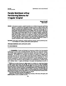
Figure 1. The three phases of the multilevel graph partitioning paradigm.

phase, in which the sequence of successively approximate graphs (coarser) is obtained, the initial partitioning phase, in which the smallest graph is partitioned, and the uncoarsening and refinement phase, in which the solution of the smallest graph is projected to the next level finer graph, and at each level an iterative refinement algorithm is used to further improve the quality of the partitioning. The various phases of multilevel approach in the context of graph bisection are illustrated in Figure 1. A commonly used method for graph coarsening is to collapse together the pairs of vertices that form a matching. A matching of the graph is a set of edges, no two of which are incident on the same vertex. Vertex matchings can be computed by a number methods, such as random matching, heavy-edge matching [17], maximum weighted matching [8], and approximated maximum weighted matching (LAM) [24]. A class of partitioning refinement algorithms that are effective in quickly refining the partitioning solution during the uncoarsening phase are those based on variations of the Kernighan-Lin and Fiduccia-Mattheyses algorithms [13, 1, 5, 19, 18, 10]. This paradigm was independently studied by Bui and Jones [2] in the context of computing fill-reducing matrix reordering, by Hendrickson and Leland [13] in the context of finite element mesh-partitioning, and by Hauck and Borriello [11] (called Optimized KLFM), and by Cong and Smith [4] for hypergraph partitioning. Karypis and Kumar extensively studied this paradigm in [16, 15, 19] for the partitioning of graphs. They presented novel graph coarsening schemes and they showed both experimentally and analytically that even a good bisection of the coarsest graph alone is already a very good bisection of the original graph. These coarsening schemes made the overall multilevel paradigm

very robust and made it possible to use simplified variants of KL or FM refinement schemes during the uncoarsening phase, which significantly speeded up the refinement process without compromising overall quality. Multilevel recursive bisection partitioning algorithms are available in several public domain libraries, such as Chaco [14], METIS [16], and SCOTCH [25], and are used extensively for graph partitioning in a variety of domains.

3

Motivation

The success of the multilevel graph partitioning algorithms is primarily due to the synergy of the coarsening and refinement phases. In particular, a good coarsening scheme can hide a large number of edges on the coarsest graph. By reducing the exposed edge weight, the task of computing a good quality partitioning becomes easier. For example, a worst case partitioning (i.e., one that cuts every edge) of the coarsest graph will be of higher quality than the worst case partitioning of the original graph. Also, a random bisection of the coarsest graph will tend to be better than a random bisection of the original graph. Similarly, being able to perform refinement at different coarse representations of the same graph significantly increases the power of partitioning refinement algorithms – allowing them to climb out of local minima by moving groups of vertices at a time. However, the effectiveness of the coarsening schemes employed by current state-of-the-art multilevel graph partitioning algorithms dramatically diminishes in the context of power-law graphs. This is because existing coarsening schemes depend on being able to find sufficiently large vertex matchings to obtain a non-trivial fractional reduction on the number of vertices in successively coarser graphs. Graphs arising in traditional scientific computing applications tend to produce such matchings. In most cases, the size of the matching is very close to half the number of vertices (i.e., most of the vertices get matched with other vertices), resulting in graph size reductions that are very close to a factor of two. On the other hand, in power-law graphs, because of the uneven degree distribution, there are a large number of lowdegree vertices attached to a relatively few high-degree vertices that dramatically limits the size of the matchings that can be computed. This is because as soon as a high-degree vertex gets matched, it cannot get matched with another vertex in the current level. This inability of the matchingbased coarsening approach to find sufficiently large matchings, has two important implications. First, the number of exposed edges tend to shrink at a very slow rate— eliminating a key advantage of the multilevel paradigm. Second, the size of successively coarser graphs does not reduce quickly—increasing the amount of memory required to store these graphs. As a result, the coarsening is usually terminated at a much earlier point (otherwise the memory

Ratio of number of vertices to initial number of vertices

1

Actor Google Auto

0.8

0.6

0.4

0.2

0 0

5

10 15 Coarsen level

20

Ratio of number of edges to initial number of edges

(a) 1

Actor Google Auto

0.8

4

0.6

0.4

0.2

0 0

5

10

15

20

Coarsen level

(b) Ratio of exposed edge weight to initial exposed edge weight

than the original one only by a constant factor. Figure 2 illustrates these points by comparing three key parameters of the coarsening history of three graphs (Google, Actor, and Auto). The parameters are the number of vertices, number of edges, and the exposed edge weight of the successively coarser graphs. Among the three graphs, the first two correspond to power-law graphs whereas the third one corresponds to a graph obtained from a 3D finite element mesh. These plots illustrate that unlike the meshbased graph for which all three parameters decrease rapidly during the course of coarsening, these parameters tend to decrease very slow and only by a small factor for the powerlaw graphs. These results suggest that in order to leverage the key concepts and power of the multilevel graph partitioning paradigm for power-law graphs, new coarsening methods need to be developed that do not exhibit the limitations of current matching-based approaches.

1

Actor Google Auto

0.8

0.6

0.4

0.2

0 0

5

10 15 Coarsen level

20

(c)

Figure 2. The reduction on (a) the number of vertices, (b) the number of edges, and (c) the exposed edge weight during the coarsening process for two power-law graphs (Google and Actor) and a finite element-based graph.

complexity of these schemes will be quadratic on the number of vertices), resulting in a graph whose size is smaller

Clustering Coarsening Schemes

The approach that we took in order to correct the limitations of matching-based coarsening schemes is to allow arbitrary size sets of vertices to be collapsed together. By doing so, we try to directly attack the source of the problem and ensure (up to a point) that the size of each successive coarser graph will decrease by a non-trivial fraction. Since our goal is to produce a sequence of successively coarser graphs that are both smaller and also have a much smaller exposed edge-weight, the problem of finding the sets of vertices to be collapsed together can be thought of as a special case of finding a large number of small and highly connected subgraphs. Finding such subgraphs is a well-studied problem in the context of graph-based clustering in data-mining [6] and a number of algorithms have been developed for solving it. However, one of our initial design considerations was to develop coarsening schemes whose complexity is not significantly higher than that of existing matching-based schemes. For this reason, the primary focus of our research was on developing rather simple but fast clustering approaches. Towards this goal we considered extensions of the heuristic matching-based algorithms that allow the discovery of arbitrary size subgraphs. The operation of most of the existing matching-based schemes can be summarized as follows [27]. They use a certain policy to order the edges of the graph and consider them for inclusion in the matching based on this ordering. For each edge (v, u) that they consider, if both v and u are unmatched, then the pair of vertices gets matched with each other and are combined in the next level coarser graph. However, if either v or u has already been matched with another vertex, then this edge is ignored and it does not contribute to the matching. If after considering all edges, some

vertices remain unmatched, then they are just copied to the next level coarser graph. Within this framework, all the methods that we consider in this paper allow an unmatched vertex v to potentially be matched with one of its adjacent vertices u even if u has already been matched. By allowing this, we essentially associate v with the cluster of vertices that u belongs to; thus, incrementally constructing the various clusters of vertices that will form the nodes of the next level coarser graph. Specifically, we consider a number of algorithms that differ along two orthogonal dimensions. The first is the overall strategy that is used to visit the edges of the graph and second is the scheme that is used to order the edges within each strategy—giving a preference to certain clusterings over others.

4.1

Edge Visiting Strategies

We consider two general strategies for visiting the various edges of the graph during the process of identifying the clusters of vertices to collapse together. These strategies will be referred to as the globally greedy strategy (GG) and as the globally random-locally greedy strategy (GRLG). For the rest of the discussion we assume that there is a function to order a set of edges E in some preference order F(E). These functions will be described later in Section 4.2, but the motivation behind them is to allow the coarsening algorithms to identify clusters of highly connected vertices. Algorithms that follow the GG strategy will order all the edges of G = (V, E) according to F(E) and then visit them based on this ordering. The motivation behind this strategy is to fully take advantage of the information encapsulated in the selected preference order by allowing the algorithm to consider for grouping together vertices that are most likely to be part of a good cluster. On the other hand, algorithms that follow the GRLG strategy will visit the vertices of the graph in a random order and for each vertex v they will use F to locally order the edges I(v) that are incident on v. The motivation behind this strategy is to eliminate the potentially expensive step of computing a global ordering of all the edges but still retain key elements of the greedy nature of the GG strategy. Additional Considerations A potential problem that can arise with the above schemes is that they may end up constructing a relatively small number of rather large clusters. As a result, the number of vertices of the successively coarser graphs can decrease by a factor that is much greater than two. Such rapid coarsenings can adversely impact the effectiveness of multilevel refinement, as the number of levels that it operates on can be small. The GG and GRLG strategies overcome this problem by employing two constraints.

First, during the cluster discovery process, both the GG and GRLG strategies keep track of the current number of vertices in the next-level coarser graph. That is, the size of the graph assuming that no further clustering has been performed and any unmatched vertices were simply copied to the coarser graph. If that size drops below half of the size of the current graph, no further clustering gets performed, and the next-level coarser graph is constructed from the current information. This constraint ensures that the size of successive coarser graphs decreases by at most a factor of two. Second, they set a limit on the size of the cluster that can be formed anywhere during the coarsening process. This limit is specified in the form of a maximum vertex weight (MaxVWgt) that any cluster can have. During the coarsening phase, if an edge will result in the creation of a cluster whose size is greater than MaxVWgt, then that particular cluster does not get formed and the edge is skipped. The value of MaxVWgt is set to be 1/20th of the total vertex weight of the original graph, which essentially limits the size of the coarsest graph at least 20 vertices. The effect of this constraint is two fold: (i) it throttles the coarsening rate, and (ii) it ensures that the size of the coarsest vertices do not become so large so that it will be infeasible to compute a balanced two-way partitioning.

4.2

Edge Ordering Criteria

Our experience with multilevel graph partitioning algorithms in the context of scientific computing applications [15] showed that the effectiveness of the various matching schemes was related with (i) their ability to collapse together regions of the graph that corresponded to well-connected subgraphs and (ii) their ability to produce coarser graphs whose vertices have a relatively uniform size distribution. Guided by these two principles we developed a number of different ordering criteria that combine various pieces of information. This information is obtained by either analyzing each edge in the context of its local environment (i.e., the edge and its incident vertices) or in a somewhat larger context derived by taking into account certain aspects of its nearby topology. Local Environment For each edge e = (v, u) we considered three pieces of information that can be obtained by analyzing e, v, and u. These are the weight of the edge (w(e)), the weight of the vertices (w(v) and w(u)), and the degree of the vertices (d(v), d(u)). The weight of the edge is important because it provides information about the strength of the connection between vertices v and u. In addition, since during the coarsening process, the weights of the edges are set to be equal to the sum of the weights of the edges of the original graph that

connect vertices encapsulated in v with vertices encapsulated in u, they provide important information on whether or not the subgraph obtained by combining v and u is wellconnected. Thus, everything else being equal, we will prefer edges that have high edge-weight over edges that do not. Note that this is also the primary motivation behind the heavy-edge matching scheme used in existing matchingbased coarsening schemes. The sum of the weights (w(v) + w(u)) is important as it affects the size distribution of the vertices in the coarser graphs. In particular, if w(v) + w(u) is very high, then this will decrease the effectiveness of the KL/FM-type refinement algorithms as it will prevent them from moving it across the partition boundary (assuming that such moves improve the cut). The reason for this is that due to its size, such a move may lead to a highly unbalanced (i.e., infeasible) bisection. Thus, everything else being equal, we will prefer edges whose sum of vertex weights is small. The degree of each vertex is important as it provides information as to how many other edges exist in the graph that can be used to cluster either v or u. For example, if min(d(v), d(u)) is one, then this edge is the only way by which one of the vertices can be included in a cluster. Everything else being equal, we should prefer edges that have at least one vertex with a very small degree as such edges provide the best (and in many cases the only) opportunity for the low degree vertex to be included in a cluster. Note that if such edges are not been given priority, by the time they will end up being considered, it may be that the size of the resulting cluster will have grown too large, preventing the formation of this cluster. Non-local Environment To obtain information about the non-local environment of each edge we use the concept of the graph core, which was first introduced by Seidman [26]. Given a graph, G = (V, E), a subgraph H induced by C ⊆ V is a core of order k, written as Hk , iff for every v ∈ C, dH (v) ≥ k, where dH (v) is the degree of vertex v in H. The core number of a vertex v (Γ(v)) is the maximum order of a core that contains that vertex. Cores exhibit the following two properties [29]: (i) for i < j, Hj ⊂ Hi (nested relation), and (ii) for each core i, Hi can contain more than one connected component. The core number of a vertex v and the properties of the cores provide information as to whether an edge e = (v, u) is part of well-connected subgraph or not. In particular, due to the nested relation, for every edge e = (v, u) we know that there is an induced subgraph that contains e whose minimum degree is at least min(Γ(v), Γ(u)). Thus, everything else being equal, we will prefer edges that have high core numbers, or edges whose core numbers are comparable. The reason why the second set of edges are of interest is because they represent some of the best potential clusters of

Globally Greedy Strategies Ordering schemes for edges e = (v, u) Coarsen Scheme Description Order Sort list of edges by GDCS 1. d(v) + d(u) Asc 2. w(e) Desc GFC 1. w(e) Desc 2. w(u) + w(v) Asc GHELD 1. w(e) Desc 2.
d(v) + d(u)
Asc GCORE 1. (Γ(u)) + (Γ(v)) Desc 2. w(e) Desc GFCDC 1. w(e) Desc 2. w(v) + w(u) Asc 3. |Γ(u) − Γ(v)| Asc GFCC 1. w(e) Desc 2. w(u) + w(v) Asc 3. Γ(u) + Γ(v) Desc Globally Random, Locally Greedy Strategies Schemes to order the edges e = (v, u) incident on v Coarsen Scheme Description Order LDHE 1. d(u) Minimum 2. w(e) Maximum HELD 1. w(e) Maximum 2. d(u) Minimum FC 1. w(e) Maximum 2. w(u) Minimum FCC 1. w(e) Maximum 2. w(u) Minimum 3. Γ(u) Maximum FCDC 1. w(e) Maximum 2. w(u) Minimum 3.
|Γ(u) − Γ(v)| Minimum
CORE 1. (Γ(u)) + (Γ(v)) Maximum 2. w(e) Maximum

Table 1. The various coarsening schemes developed by combining different edge visiting strategies and ordering criteria.

the vertices involved. Note that the notion of the graph core has been extended beyond just the degree of a vertex to also include more general functions such as the sum-of-the-edge-weights [29]. Since we are dealing with weighted graphs, we used this latter core numbering definition. Note that there is a O(|E|)time algorithm to compute the core numbering in the context of degrees [28] and a O (|E| max (∆, log |V |))-time algorithm, where ∆ is the maximum degree of the graph, for the case of the sum-of-the-edge-weights [29].

4.3

Putting Everything Together

A large number of coarsening approaches can be developed by combining the two edge visiting strategies and the four edge ordering criteria. Due to space constraints, in this paper we focus on a subset of them that our initial studies showed to represent some of the best combinations. The key

characteristics of these schemes are summarized in Table 1. Note here that the order of the criteria determines their role as the primary, secondary, or tertiary importance

5

Experimental results

5.1

Dataset Description

We evaluated the performance of the new coarsening schemes on ten different graphs obtained from various sources. The characteristics of these graphs are shown in Table 2.

Dataset Citations DBLP Actor Google NDwww Overture PPI Scan Lucent Scan+Lucent

#vertices 27400 310138 498925 198782 325729 75002 59191 228263 112969 284772

#nedges µ 352504 25.73 1024262 6.61 1460791 5.86 295063 2.97 1090107 6.69 411013 10.96 160737 5.43 320149 2.81 181639 3.22 449228 3.16

Degree σ max 45.56 2468 9.94 344 11.39 646 12.14 1471 42.82 10721 53.93 6619 12.30 1116 8.36 1937 4.93 423 9.05 1978

fit of f = αdβ α β 3.34 -7.92 6.33 -8.81 2.51 -1.89 1.35 -2.28 1.62 -5.83 3.51 -1.43 2.42 -1.55 1.34 -1.77 4.37 -1.19 1.47 -5.36

Table 2. Characteristics of the different graphs used to evaluate the multilevel partitioning algorithm.

The PPI dataset is created from Database of Interacting Proteins (DIP)5 . Each vertex in this graph corresponds to a particular protein and there is an edge between a pair of proteins if these proteins have been experimentally determined to interact with each other. The SCAN dataset corresponds to the Internet map obtained using the Mercator software. Each vertex represents an Internet router and an edge implies that the two routers at the endpoints are adjacent. The Lucent dataset was constructed via tracerouters collected by the Internet Mapping project at Lucent laboratories. Each vertex represents a router and an edge indicates adjacency between the routers. The SCAN+Lucent dataset was obtained by the merging of information from the Lucent and SCAN datasets6 . The Actor dataset was constructed from the actor data of the Internet Movie Database (IMDB)7 . Vertices represent actors and movies. Each edge has an actor as one endpoint and a movie as the other and indicates that the actor played in the movie. Since the original version of the above datasets contained a large number of singleton vertices and/or very small connected components, we first extracted from each dataset the largest connected component and used it for our evaluation. The statistics presented in Table 2 correspond to the largest connected component and not the original dataset.

5.2 The Citation dataset was created from the citation graph used in KDD Cup 20031 . Each vertex in this graph corresponds to a document and each edge corresponds to a citation relation. Because the partitioning algorithms deal with undirected graphs, the direction of these citations was ignored. The DBLP dataset was created from the coauthorship information from Computer Science research publications2 . Vertices in the graph represent authors and edges exist if a pair of authors have co-authored at least one publication. The Google dataset was obtained from the 2002 Google Programming Contest3 . The original dataset contains various web-pages and links from various “edu” domain. We converted the dataset into an undirected graph in which each vertex corresponds to a web-page and an edge to a hyperlink between web-pages. In creating this graph, we kept only the links between “edu” domains that connected sites from different subdomains. The NDwww dataset is a complete map of the nd.edu domain4 . Each vertex represents a web page and an edge represents a link between two pages. The Overture dataset was obtained from Overture Inc (now part of Yahoo!) and is similar in nature to the Google dataset and corresponds to a three-level deep crawl out of ten seed CS homepage of major Universities. 1 http://www.cs.cornell.edu/projects/kddcup/datasets.html 2 http://www.informatik.uni-trier.de/

ley/db/index.html 3 http://www.google.com/programming-contest/ 4 http://www.nd.edu/ networks/resources.htm

Experimental Methodology

Since many of the schemes under consideration are randomized in nature, in order to ensure that the results are not biased in any way, we computed 100 different bisections for each graph and report the average cuts. In the case of the schemes following the GRLG strategy, each different run was performed using a different randomly obtained ordering of the vertices. In the case of the GG strategies, randomization was introduced as a tie-breaking mechanism. Furthermore, in running the experiments we set the load imbalance to zero thus ensuring a perfect balance among the partitions (i.e. equal partition weights). For example, for two-way partitioning, the weight of each partition will equal half the total vertex weight. The performance of the different schemes presented in this paper were compared against two existing partitioning algorithms. The first is the bisection algorithm provided by METIS [16] (using the pmetis program) and the second is the spectral partitioning algorithm provided by Chaco [14]. Note that the bisections produced by spectral were further refined by using a KL refinement algorithm (i.e., the SPECTRAL-KL option of Chaco). Note that due to space constraints, our experimental evaluation was limited to only two-way partitionings. However, 5 http://dip.doe-mbi.ucla.edu/ 6 All three of these datasets can be http://www.isi.edu/div7/scan/mercator/maps.html. 7 http://www.nd.edu/ networks/resources.htm.

obtained

from

the relative performance of the different schemes remains the same for larger number of partitions.

5.3

Results

The cuts obtained by the various schemes across the different datasets are shown in Table 3. This table shows the performance of 12 different schemes, the ten introduced in this paper and described in Table 1 along with the performance achieved by METIS and Spectral. The last row of the table contains the minimum cut achieved over the different schemes, whereas the last column (labeled “ACRB”) shows the Average Cut Relative to the Best. For a particular scheme, this measure is obtained by computing the ratio of the cut obtained on a particular graph over the minimum cut obtained by the different schemes, averaged over the different datasets. The value of ACRB will be greater than or equal to one. A value close to one indicates that a particular scheme obtains cuts that are either the smallest or very close to the smallest obtained, whereas a large value indicates that the cuts obtained by a scheme are much worse than the best cuts obtained by the different schemes. In addition to the direct cut-based comparisons, Table 4 compares the various schemes by analyzing the extent to which the difference in performance between each pair of schemes is statistically significant or not. For our statistical significance testing we used the Wilcoxon’s paired signed rank test at 5% significance level. The entries marked with “”) indicate that the scheme of the row performs statistically worse (better) than the scheme of the column. Entries marked with “=” indicate that the difference between the two schemes is not statistically significant. Note that the last column (labeled “Win-Loses”) displays the difference between the number of schemes in which a particular scheme is statistically better and the number of schemes in which the scheme is statistically worse. Thus, a positive value indicates a scheme that does well whereas a negative value represents a scheme that does poorly. Discussion Looking at the results from these tables we can make a number of observations. First, comparing the GG with the GRLG strategies we can see that the GG schemes do not perform as well as the GRLG ones. The best globally greedy scheme has an ACRB value of 1.57 as compared to the best locally greedy ACRB value of 1.06. Moreover, the advantage of GRLG over GG is also statistically significant. In fact almost all GRLG schemes outperform the GG schemes. Second, comparing ordering schemes that use local information against schemes that also incorporate non-local information provide by the core numbering, we can see that core numbering alone leads to poorly performing schemes (e.g., CORE/GCORE). However, the combination of local information with core numbering leads to improved results.

In fact, the FCDC, which is the best performing scheme in terms of ACRB combines information about the edge weight, vertex weights, and cores. However, the difference between FCDC and FC (which uses only edge- and vertexweights) is not statistically significant. Third, comparing the performance achieved by the various schemes proposed in this paper, we can see that three of them, FCDC, FC, and HELD produce results that are quite comparable (the schemes are not statistically different from each other) and are the best performing schemes. Fourth, comparing the performance achieved by the above three schemes against that achieved by METIS and Spectral, we can see that all three of them produce results that are substantially better than either one of them. Also, in addition to the above three schemes, METIS is also being outperformed by FCC, whereas Spectral is also outperformed by FCC and LDHE. Finally, to illustrate how the coarsening schemes developed in this paper overcome the limitations of the matchingbased coarsening schemes described in Section 3, Figure 3 shows the rate at which the number of vertices, number of edges, and the exposed edge-weight decreases for the FC coarsening scheme and the heavy-edge matching-based (HEM) scheme for Google and Actor. Note that the results for HEM are identical to those shown in Figure 2. As we can see from these plots, the coarsening schemes are quite effective in producing successive coarser graphs in which all three of these quantities reduce at a much higher rate than HEM.

6

Conclusions and Directions for Future Research

This paper focused on the problem of developing graph partitioning algorithms for power-law graphs. Towards this goal it presented a number of new algorithms based on the multilevel graph partitioning paradigm that were designed to leverage the strengths inherent to these approaches and to address the challenges imposed due to the uneven degree distribution of these graphs. The comprehensive experimental evaluation presented in this paper showed that three of the methods introduced in this paper achieve consistently some of the best results, outperforming both existing state-of-the-art multilevel methods as well as more traditional partitioning approaches based on spectral methods. The research in this paper can be extended along a number of directions including the development of even better coarsening schemes as well as the development of effective parallelization strategies for them. We expect that existing approaches used to parallelize serial multilevel graph partitioning algorithms can be easily extended for the context of the new coarsening schemes. In addition, one of the issues that need to be further investigated is the extent to which the

FC FCDC HELD FCC LDHE GCORE GDCS GFC GFCDC GHELD CORE GFCC METIS Spectral Minimum

Citations DBLP Actor Google NDwww Overture PPI Scan Lucent Scan+Lucent ACRB 17122 51972 42376 6791 1813 25855 9286 4404 2378 7779 1.07 15868 52405 42404 6867 1866 26029 8926 4560 2387 7594 1.06 20264 51967 40000 6725 1863 25740 8845 4370 2490 7762 1.08 17836 53246 42985 6913 1827 26498 9226 4537 2464 7829 1.09 22829 55387 39762 7159 3546 26321 9772 6019 2904 10176 1.31 15196 56923 57796 10934 8121 30752 11535 5817 3754 10291 1.69 23786 56628 40809 8006 6425 28044 10177 7096 3142 11889 1.57 15191 71846 51568 8922 5410 30073 10552 7847 3699 12343 1.59 15503 71347 51776 10395 9480 27992 10272 7409 3673 11905 1.80 28395 61672 49103 7540 6270 32046 10529 7953 3096 12563 1.66 23466 80620 47579 13506 9505 33141 12629 7604 4908 13957 2.05 14914 85087 50714 19596 10610 34036 13788 15747 5039 24463 2.54 14925 61242 113962 14758 6638 34973 12853 11575 4323 6411 1.94 25765 72450 78342 7144 8120 33588 7469 4950 3874 22047 1.91 14914 51967 39762 6725 1813 25740 7469 4370 2378 6411

Table 3. The edge-cuts of the different coarsening schemes averaged over 100 runs.

FC FCDC HELD FCC LDHE GCORE GDCS GFC GFCDC GHELD CORE GFCC METIS Spectral

FC FCDC HELD FCC LDHE GCORE GDCS GFC GFCDC GHELD CORE GFCC METIS Spectral Win-Loses = = = > > > > > > > > > > > 11 = = = > > > > > > > > > > > 11 = = = = > > > > > > > > > > 10 < < = = = > > > > > > > > > 7 < < < = = = > > > > > > = > 4 < < < < = = = = = = = > = = -3 < < < < < = = = = > > > = = -2 < < < < < = = = = = > > = = -3 < < < < < = = = = = > > = = -3 < < < < < = < = = = = = = = -6 < < < < < = < < < = = = = = -8 < < < < < < < < < = = = = = -9 < < < < = = = = = = = = = = -4 < < < < < = = = = = = = = = -5

Table 4. Results of statistical significance testing using Wilcoxon’s paired signed rank test using 5% significance level.

information provided by the cores can also be used to improve the performance of traditional matching-based coarsening schemes. Acknowledgment This work was supported in part by NSF EIA-9986042, ACI-0133464, ACI-0312828, and IIS-0431135; the Digital Technology Center at the University of Minnesota; and by the Army High Performance Computing Research Center (AHPCRC) under the auspices of the Department of the Army, Army Research Laboratory (ARL) under Cooperative Agreement number DAAD19-01-2-0014. The content of which does not necessarily reflect the position or the policy of the government, and no official endorsement should be inferred. Access to research and computing facilities was provided by the Digital Technology Center and the Minnesota Supercomputing Institute.

[4]

[5]

[6] [7]

[8]

References [1] C. Ashcraft and J. Liu. Using domain decomposition to find graph bisectors. Technical report, York University, North York, Ontario, Canada, 1995. [2] T. Bui and C. Jones. A heuristic for reducing fill in sparse matrix factorization. In 6th SIAM Conf. Parallel Processing for Scientific Computing, pages 445–452, 1993. [3] U. Catalyurek and C. Aykanat. Hypergraph-partitioning based decomposition for parallel sparse-matrix vector mul-

[9]

[10]

tiplication. IEEE Transactions on Parallel and Distributed Systems, 10(7):673–693, 1999. J. Cong and M. L. Smith. A parallel bottom-up clustering algorithm with applications to circuit partitioning in vlsi design. In Proc. ACM/IEEE Design Automation Conference, pages 755–760, 1993. R. Diekmann, B. Monien, and R. Preis. Using helpful sets to improve graph bisections. In D. Hsu, A. Rosenberg, and D. Sotteau, editors, Interconnection Networks and Mapping and Scheduling Parallel Computations, volume 21, pages 57–73. AMS Publications, DIMACS Volume Series, 1995. R.O. Duda, P.E. Hart, and D.G. Stork. Pattern Classification. John Wiley & Sons, 2001. C. M. Fiduccia and R. M. Mattheyses. A linear time heuristic for improving network partitions. In In Proc. 19th IEEE Design Automation Conference, pages 175–181, 1982. H. Gabow. Data structures for weighted matching and nearest common ancestors with linking. In Proc. of the 1st Annual ACM-SIAM Symposium on Discrete Algorithms, pages 434–443, 1990. Ananth Grama, Anshul Gupta, George Karypis, and Vipin Kumar. Introduction to Parallel Computing: Design and Analysis of Algorithms, 2nd Edition. Adison Wesley Publishing Company, Redwood City, CA, 2003. W. Hager, S. Park, and T. Davis. Block exchange in graph partitioning. In P. Pardalos, editor, Approximation and Complexity in Numerical Optimization: Continuous and Discrete

Ratio of number of vertices to initial number of vertices

1

Actor[FC] Google[FC] Actor[HEM] Google[HEM]

0.8

0.6

0.4

0.2

0 0

5

10 15 Coarsen level

20

Ratio of number of edges to initial number of edges

(a) 1

Actor[FC] Google[FC] Actor[HEM] Google[HEM]

0.8

0.6

0.4

0.2

0 0

5

10 15 Coarsen level

20

Ratio of exposed edge weight to initial exposed edge weight

(b) 1

Actor[FC] Google[FC] Actor[HEM] Google[HEM]

0.8

0.6

0.4

0.2

0 0

5

10 15 Coarsen level

20

(c)

Figure 3. The reduction on (a) the number of vertices, (b) the number of edges, and (c) the exposed edge weight during the coarsening process for two power-law graphs (Google and Actor) using coarsening schemes FC and HEM.

Problems. Kluwer Academic Publishers, 1999.

[11] S. Hauck and G. Borriello. An evaluation of bipartitioning technique. In Proc. Chapel Hill Conference on Advanced Research in VLSI, 1995. [12] B. Hendrickson. Graph partitioning and parallel solvers: Has the emperor no clothes? In Proc. Irregular’98, pages 218– 225, 1998. [13] Bruce Hendrickson and Robert Leland. A multilevel algorithm for partitioning graphs. Technical Report SAND931301, Sandia National Laboratories, 1993. [14] Bruce Hendrickson and Robert Leland. The chaco user’s guide, version 2.0. Technical Report SAND94-2692, Sandia National Laboratories, 1994. [15] G. Karypis and V. Kumar. Analysis of multilevel graph partitioning. In Proceedings of Supercomputing, 1995. [16] G. Karypis and V. Kumar. Technical report, Department of Computer Science, University of Minnesota, 1998. [17] G. Karypis and V. Kumar. A fast and high quality multilevel scheme for partitioning irregular graphs. SIAM Journal on Scientific Computing, 20(1):359–392, 1998. [18] G. Karypis and V. Kumar. Multilevel k-way partitioning scheme for irregular graphs. Journal of Parallel and Distributed Computing, 48(1):96–129, 1998. [19] G. Karypis and V. Kumar. A fast and highly quality multilevel scheme for partitioning irregular graphs. SIAM Journal on Scientific Computing, 20(1), 1999. [20] B. W. Kernighan and S. Lin. An efficient heuristic procedure for partitioning graphs. The Bell System Technical Journal, 49(2):291–307, 1970. [21] J. Kleinberg. Authoritative sources in a hyperlinked environment. In Proc. of the Nineth Annual ACM-SIAM Symposium on Discrete Algorithms, 1998. [22] R. Tanaka J.C. Doyle W. Willinger L. Li, D. Alderson. Towards a theory of scale-free graphs: Definition, properties, and implications. Technical Report CIT-CDS-04-006, California Institute of Technology, Pasadena, CA, 2004. [23] R. Motwani T. Winograd L. Page, S. Brin. The pagerank citation ranking: Bringing order to the web. Technical report, Stanford Digital Library Technologies Project, 1998. [24] B. Monien, R. Preis, and R. Diekmann. Quality matching and local improvement for multilevel graph-partitioning. Technical report, University of Paderborn, 1999. [25] F. Pellegrini and J. Roman. SCOTCH: A software package for static mapping by dual recursive bipartitioning of process and architecture graphs. HPCN-Europe, Springer LNCS 1067, pages 493–498, 1996. [26] Seidman S.B. Network structure and minimum degree. Social Networks, 5:269–287, 1983. [27] Kirk Schloegel, George Karypis, and Vipin Kumar. Graph partitioning for high-performance scientific simulations. In Jack Dongara, Ian Foster, Geoffrey Fox, William Gropp, Ken Kennedy, Linda Torczon, and Andy White, editors, Sourcebook on Parallel Computing, chapter 18, pages 491–541. Morgan Kaufmann, San Francisco, CA, 2002. [28] M. Zaver˘snik V. Batagelj. An O(m) algorithm for cores decomposition of networks. [29] M. Zaver˘snik V. Batagelj. Generalized cores. Journal of the ACM, V(N):1–8, 2002.