Article Cite This: Ind. Eng. Chem. Res. 2017, 56, 13800-13811
pubs.acs.org/IECR
Multimode Continuous Processes Monitoring Based on Hidden SemiMarkov Model and Principal Component Analysis Zhijiang Lou† and Youqing Wang*,‡,† †
College of Information Science and Technology, Beijing University of Chemical Technology, Beijing 100029, China College of Electrical Engineering and Automation, Shandong University of Science and Technology, Qingdao 266590, China
‡
ABSTRACT: Several studies have applied the hidden Markov model (HMM) in multimode process monitoring. However, because the inherent duration probability density of HMM is exponential, which is inappropriate for modeling the multimode process, the performance of these HMM-based approaches is not satisfactory. As a result, the hidden semi-Markov model (HSMM), which integrated the mode duration probability into HMM, is combined with principal component analysis (PCA) to handle the multimode feature, named as HSMMPCA. PCA is a powerful monitoring algorithm for the unimodal process, and HSMM specializes in mode division and identification. HSMM-PCA inherits the advantages of these two algorithms and hence it performs much better than the existing HMM-based approaches do. In addition, HSMM-PCA can detect the mode disorder fault, which challenges the most multimode approaches.
1. INTRODUCTION To ensure the process safety and deliver of high quality consistent product, process monitoring is of critical importance for the chemical industry. In recent years, with the fast development of computer and information technologies, a massive amount of process history data is available for abnormal conditions detection. As a result, multivariate statistical process control (MSPC) methods,1,2 which only require historical process data, are becoming more and more popular in large-scale chemical industries. As one of the most popular MSPC methods, principal component analysis (PCA)3−5 has been successfully applied in online continuous process monitoring, and a great quantity of advanced PCA approaches have been put forward in literature.6−9 One basic assumption for PCA is that the normal data should come from a single operation region; i.e., the process data obey unimodal Gaussian distribution. In reality, due to various factors, such as the alterations of feedstock and compositions, the changing of manufacturing strategies, and the disturbance in the external environment, usually the industry processes work at multiple operating modes and hence this assumption is invalid. As a result, the process mode is not fixed and it shifts from one mode to another, which confines the application of the traditional PCA approaches. To address the multimode problem, three kinds of approaches have been put forward: (1) global model approach, which builds one uniform model to fit all modes;10 (2) the multimode approach, which divides the entire process into different stages by using the clustering algorithms and then builds the corresponding sub-PCA model for each stage separately;11,12 (3) the mixture model approach, which © 2017 American Chemical Society
combines different PCA models for process approximation.13−15 In recent years, many research efforts have been done on the basis of these approaches, and a lot of papers have been published.16,17 All these above-mentioned approaches have one common drawback; i.e., they do not take the mode shifting probability into consideration. For most chemical industry processes, usually their operating sequences are fixed and hence the current operation mode probabilistically depends on the last operation mode. Without the restriction of mode shifting probability, in the offline modeling stage, these multimode approaches may falsely divide the operation modes and build the wrong PCA model for each mode, and in the online monitoring stage, they may obtain the wrong mode localization result. The hidden Markov model (HMM),18−20 which was first developed by Baum and his co-workers, has gained great success in a wide range of fields, such as speech recognition and bioinformatics. HMM contains a finite number of hidden states and each hidden state emits one observation; moreover, each hidden state shifts to other states with a certain probability, called the state transition probability. For HMM, the hidden states can be regarded as the operation modes in the multimode process and the state transition probability can be used to describe the operation mode shifting probability, so several papers have adopted HMM to address the multimode Received: Revised: Accepted: Published: 13800
April 24, 2017 September 22, 2017 October 31, 2017 October 31, 2017 DOI: 10.1021/acs.iecr.7b01721 Ind. Eng. Chem. Res. 2017, 56, 13800−13811
Article
Industrial & Engineering Chemistry Research problem in recently years.21−25 For these papers, the major weakness is that the inherent duration probability density of HMM is exponential,26 whereas the duration of operation modes in real chemical processes usually fluctuates around a nonzero value, so HMM is inappropriate for description of the multimode processes. Another drawback of these HMM-based approaches is that they are invalid for detecting mode disorder fault. The mode disorder fault means that data in each mode are in normal condition whereas the mode shifting order is wrong. For example, for a process where mode A can only shift to mode B, when a mode shifting disorder fault occurs (mode A directly shift to mode C), these HMM-based approaches just adopt the most suitable mode model (mode C) to monitor the process data. Without the restriction that mode A cannot shift to mode C directly, these methods cannot detect this abnormal condition, because the data in mode C are normal. As an extended model of HMM, the hidden semi-Markov model (HSMM)27−29 introduces the state duration probability matrix to describe the time spent in a given operation mode, so HSMM has a better ability to describe multimode processes. In papers,30,31 Chen and Jiang first combined HSMM with two improved PCA approaches and hence achieved MPCA-HSMM and DMPCA-HSMM for monitoring multimode batch processes. The main ideas of MPCA-HSMM and DMPCAHSMM are similar: preprocessing the whole process data by using PCA and then monitoring the uncorrelated principal components with HSMM. However, PCA is a unimode algorithm, so it may fail in extracting the uncorrelated principal components in different operation modes.32 To address this issue, this article exchanged the order of HSMM and PCA, and proposed a new combination of PCA and HSMM (HSMMPCA). In HSMM-PCA, HSMM is used for dividing and identifying the process modes first, and then PCA is adopted for monitoring the data in each operation mode. The greatest advantage of HSMM-PCA is that it adopts the mode affiliation information on the historical data, the mode shifting probability, and the mode duration probability for mode identification, and hence it can detect the mode disorder fault in multimode process, which is validated by the simulation in the modified TE process. The characteristics of the traditional multimode approaches, the existing HMM-based approaches, and HSMM-PCA are summarized as in Table 1.
Tennessee Eastman (TE) simulation process33 and its comparison with the existing multimode approaches; finally, conclusions are drawn in section 6.
2. PRELIMINARIES This section briefly reviews two algorithms, HSMM and PCA, as a prelude to the proposed approach. 2.1. Hidden Semi-Markov Model. HSMM is an extension of HMM, and generally speaking, HSMM can be regard as a HMM with explicit state duration probability distributions. HSMM represents a stochastic sequence, where the states are unobservable, but each state generates a sequence of observations according to a probability distribution, so these states are called as hidden states. The key elements in HSMM are as follows: (1) the discrete hidden states S = {S1, S2, ···, SM}, where M denotes the number of possible hidden states in the whole process (2) the state transition probability matrix A = {aij} (1 ≤ i, j ≤ M), where aij = P(q(t+1) = Sj | q(t) = Si) denotes the transition probability from state Si to the state Sj, and q(t) ∈ {S1, S2, ···, SM} denotes the hidden state at time t (3) the initial state probability vector π = {πi}, where πi = P(q(1)=Si) (4) the state duration probability distribution matrix Di(T ) = P(q(t +1) = Si , ···, q(t +T −1) = Si , q(t +T ) ≠ Si|q(t ) = Si , q(t −1) ≠ Si)
where T ∈ {1, 2, ···, Tmax} denotes the duration of the hidden state, and Tmax is the maximum amount of time spent in each state (5) the observations o(t) (t = 1, 2, ···, Ttotal), where Ttotal denotes the total number of observations in the process (6) the observations probability distribution Bi(o(t)) = P(o(t) | q(t) = Si), which indicates that the output at time t depends only on the corresponding hidden state qt Take λ = (A, π, {Bi}, {Di}) as the set of whole model parameters, and they can be estimated by the forward− backward algorithm, which can be found in detail in ref 34. Then one can calculate the joint probability as follows: ςi(t ) = P(o(1), o(2), ···, o(Ttotal), q(t ) = Si|λ)
Table 1. Characteristics of Various Multimode Approaches information of mode shifting probability traditional multimode approaches existing HMMbased approaches proposed HSMM-PCA
duration distribution
not been used
Further, the state affiliation probability γi(t) can be obtained as
detect mode disorder fault
γi(t ) = P(q(t ) = Si|λ , o(1), o(2), ···, o(Ttotal))
been used in both mode division and identification
(
incapable
= only been used in mode division
restricted to exponential distribution no restriction
(1)
incapable
⎛ ⎜ ⎝
P(o(1), o(2), ···, o(Ttotal), q(t ) = Si|λ) P(o(1), o(2), ···, o(Ttotal))
M ∑ j = 1 P(o(1), o(2), ···, o(Ttotal), q(t )
)
=
= Sj|λ) ⎞
P(o(1), o(2), ···, o(Ttotal))
⎟ ⎠
(2) 35
capable
And the maximum a posteriori (MAP) hidden states can be obtained as follows: q(̂ t ) = arg max ςi(t ) = arg max γi(t ) Si ,1 ≤ i ≤ M
The remainder of this paper is structured as follows. The HSMM and PCA are briefly introduced in section 2. In section 3, HSMM-PCA based process monitoring framework is discussed; then the parameter selection problem and sensitivity analysis are studied in section 4. Section 5 reports the simulation studies of the proposed approach using the modified
Si ,1 ≤ i ≤ M
ςi(t ) M ∑ j = 1 ςj(t )
estimation of the
(3)
2.2. Principal Component Analysis for Process Monitoring. PCA is a dimension reduction method that compresses the original high dimensional data into a set of lower dimensional latent variables, called the principal components (PCs). Before applying PCA, the process data 13801
DOI: 10.1021/acs.iecr.7b01721 Ind. Eng. Chem. Res. 2017, 56, 13800−13811
Article
Industrial & Engineering Chemistry Research
Figure 1. Flowchart of HSMM-PCA.
each operation mode obey unimodal Gaussian distribution, i.e., x i ∼ 5(μi ,Σi) (i = 1, 2, ···, M), where xi denotes the data belonging to mode i, and μi and ∑i are the corresponding expectation vector and covariance matrices. Set Λ̃i = diag(∑i(1,1), ∑i(2,2), ···, ∑i(s,s)), then data xi can be normalized as xĩ = (xi − μi)Λ̃i−1 and hence the corresponding principal −1 component scores ti = x̃iPi = (x i − μi )Λ̃ i Pi ∼ 5(0,Λi) (i = 1, 2, ···, M), where matrix Pi is the loading matrix of mode i and Λi is the estimated covariance matrix of ti. As a result, the observations probability distribution {Bi} can be calculated as
should be normalized to zero means and unit variance by subtracting the average of the training data and dividing by the standard deviation of the training data. Then the normalized process data matrix X ∈ Rn×s (where n is the number of samples and s is the number of variables) can be decomposed as X = TPT + E
(4)
where T ∈ R represents the score matrix, P ∈ R refers to the loading matrix, and E ∈ Rn×s is the matrix of residuals. Then PCA constructs the T2 and SPE indexes36 to monitor the principal component space and residual space spanned by T and E respectively. Statistic T2 is a measure of the principal components and statistic SPE is a measure of the approximation error. Given a normalized monitoring vector y ∈ R1×s, the T2 and SPE statistics can be computed as follows: n×ρ
s×ρ
T 2 = yP(Λ)−1PTy T
−1
Bi (x) =
(6) ρ×ρ
where I is the identity matrix; Λ = diag(λ1 ··· λρ) ∈ R is the estimated covariance matrix of principal component scores. The control limit of T2 index for a Gaussian process is (n − 1)(n + 1)ρ δT 2 = n(n − ρ) Fα(ρ ,n−ρ), where Fα (ρ,n−ρ) is an F-
distribution with ρ and (n − ρ) degrees of freedom with the level of significance α; the threshold of SPE is 1/ h0 ⎡ C h 2θ θ h (h ) ⎤ s δSPE 2 = θ1⎢ α 0θ 2 + 1 + 2 θ0 0 ⎥ , where θi = ∑ j = ρ + 1 λji , ⎣ ⎦ 1 1
h0 = 1 −
2θ1θ3 3θ2 2
M
−1
∑ j = 1 f((x−μj )Λ̅ j Pj|0,Λj)
(7)
where f(•|0,Λi) is the Gaussian probability density function with expectation 0 and variance Λi. According to eq 7, Bi(x) is calculated in the subspace of principal components rather than in the subspace of original data, so it is robust to the process noise. The detail operation in each steps are as follows: Offline modeling: Available Data: historical normal training data set X ∈ Rn×s. Step 1: Set the phase number M and the maximum duration Tmax for HSMM. Step 2: Preset the initial values as λ = (A, π, {Bi}, {Di}). Vector πi ∈ R1×Tmax (i = 1, 2, ···, M) satisfies the condition M ∑i = 1 πi = 1, matrix A ∈ RM×M can be set as a random matrix
(5)
SPE = y(I − PPT)(I − PPT)y T
f((x−μi )Λ̅ i Pi|0,Λi)
, and Cα is the normal deviate corresponding to
M
satisfying ∑ j = 1 A(i ,j) = 1 and A(i,i) = 0 for all i = 1, 2, ···, M, and vector Di(i = 1, 2, ···, M) can be set as random vectors T D (T ) = 1. Equation 7 indicates satisfying the condition ∑Tmax =1 i that observations probability distribution Bi can be described by four parameters: μi, Λ̅ i, Pi, and Λi. To obtain the initial values of these four parameters, the training data should be clustered into M groups by the k-means algorithm first, and then the corresponding μi, Λ̅ i, Pi, and Λi can be calculated for each group as the initial values of each parameter. Step 3: Use the forward−backward algorithm to re-evaluate the model parameters A, π, and {Di} and then calculate the state affiliation probability γi(t). The detailed steps of the forward−backward algorithm are as follows:
the (1 − α) percentile.
3. PROPOSED METHODOLOGY The last section has presented the preliminaries of HSMM and PCA. Because PCA is a widely acknowledged algorithm in unimodal process monitoring, and HSMM specializes in mode division and identification, this section combines them for multimode process monitoring. As shown in Figure 1, HSMM divides and identifies the process modes, and then PCA is adopted for monitoring the data in each operation mode. Before the detail introduction to each steps in HSMM-PCA scheme, the process to calculate the observations probability distribution {Bi} should be illustrated first. Assume that data in 13802
DOI: 10.1021/acs.iecr.7b01721 Ind. Eng. Chem. Res. 2017, 56, 13800−13811
Article
Industrial & Engineering Chemistry Research Step 3.1. Calculate the forward variable αi(t,T) = P(o(1), o(2), ···, o(t), q(t) = Si, τt = T) using ⎧ αi(1,T ) = πiBi (o(1)) Di(T ) ⎪ ⎪ α (t ,T ) = α (t −1,T +1) B (o(t )) i i ⎪ i ⎛ ⎞ ⎨ ⎪ + ⎜∑ αj(t −1,1)aji⎟Bi (o(t )) Di(T ) ⎜ ⎟ ⎪ ⎝ j≠i ⎠ ⎪ ⎩ t>1
Ttotal
Σi =
t=1
(8)
T
γi(̂ t ) = (9)
ξt(i ,j) = P(o(1), o(2), ⋯ , o(Ttotal), q(t −1) = Si , q(t ) = Sj) ⎞ ⎛ = αi(t −1,1)aijBj (o(t ))⎜⎜ ∑ Dj(T ) βj (t ,T )⎟⎟ ⎠ ⎝T ≥ 1
T
M
∑Tmax ∑ j = 1 αj(t ,T ) =1
(18)
M
(10)
T 2(t ) =
ηi(t ,T ) = P(o(1), o(2), ⋯ , o(Ttotal), q(t −1) ≠ Si , q(t ) = Si , τt = T )
∑ γi(̂ t ) T 2i(t )
(19)
i=1
∑ αj(t −1,1)ajiBi(o(t )) Di(T ) βi (t ,T )
M
SPE(t ) =
j≠i
(11)
∑ γi(̂ t ) SPEi(t )
(20)
i=1
and
where
ςi(t ) = P(o(1), o(2), ⋯ , o(Ttotal), q(t ) = Si)
−1 −1 Ti 2(t ) = Λ̃ i (y(t ) − μi )T Pi(Λi)−1 Pi T(y(t ) − μi )Λ̃ i
⎧ α (T ,T ), if t = Ttotal ⎪ ∑ i total ⎪T≥ 1 =⎨ ⎪ ςi(t +1) + ∑ (ξt + 1(i ,j) − ξt + 1(j ,i)), if t < Ttotal ⎪ j≠i ⎩
(21) −1
T T ̃ −1 SPEi(t ) = Λ̃ i (y(t ) − μi )T (I − PP i i )(I − PP i i )(y(t ) − μi )Λi (22)
Similarly, the control limit of T2 and SPE statistics at time t can also be approximated as
(12)
Step 3.3. Re-estimate parameters {ai,j}, {πi}, and {Di} with the respective equations: Ttotal
aî , j =
M
T 2 limit(t ) =
M Ttotal j ′= 1 t = 1
SPE limit(t ) =
Ttotal
Tmax Ttotal T ′= 1 t = 1
(15)
Step 3.4. Re-estimate parameters μi and ∑i using the following35 Ttotal
∑ γi(t ) X(t ) t=1
(24)
Equations 19−24 indicate that HSMM-PCA calculates the mode affiliation probability γ̂t(i) of each mode and then the weighted sums of all delectation results from various operation modes, as the corresponding control limits. When the data are within the normal condition, the statistics for the relevant modes are very small and the statistics for the irrelevant modes detect the fault. However, because the affiliation probability values of the irrelevant modes are close to 0, so the final statistics T2(t) and SPE(t) are still within the normal range. When a traditional fault occurs in the process, the statistics for both the relevant and irrelevant modes are larger than their
(14)
∑ ηi(t ,T )/ ∑ ∑ ηi(t ,T ′) t=1
∑ γi(̂ t )SPE limit(i) i=1
πî = ςi(1)/∑ ςj(1) j=1
(23)
M
(13)
M
Dî (T ) =
∑ γi(̂ t )Tlimit 2(i) i=1
∑ ξt(i ,j)/ ∑ ∑ ξt(i ,j′) t=1
μi =
∑Tmax α (t ,T ) =1 i
Equation 8 indicates that, αi(t,T) is calculated on the basis of αi(t−1,T), A, and {Di}, which means that the mode affiliation information on the historical data, the mode shifting probability, and the mode duration probability are used in online mode identification. Step 2: Calculate T2 and SPE statistics as
Step 3.2. Calculate the following joint probabilities:
=
(17)
Recalculate the variance of each variable as Λ̃i = diag(∑i(1,1), ∑i(2,2), ···, ∑i(s,s)). Step 3.5. Repeat steps 3.1−3.4 until all parameters converge. Step 4: Recalculate the loading matrices {Pi} and the variance matrices {Λi} for all phases i = 1, 2, ···, M. Also, compute the control limits of T2 and SPE statistics for each mode i, termed as Tlimit2 (i) and SPElimit (i). Online monitoring: Available Data: real time test data y(t) ∈ R1×s. Step 1: Estimate the mode affiliation probability γi(t). In the online monitoring stage, one cannot obtain the future data y(t′) (t′ > t) for calculation of ςi(t), and hence the forward variable αi(t,T), which only demands the historical data before time t, is used to replace ςi(t) in calculation of mode affiliation probability:
where τt denotes the remaining time of the current state q(t). Calculate the backward variable βi(t,T) = P(o(t+1), o(t+2), ···, o(Ttotal), q(t) = Si, τt = T) with formula ⎧ ⎞ ⎛ ⎪ β (t ,1) = ∑ a B (o(t +1))⎜ ∑ D (T ) β (t +1,T )⎟ ij i S ⎟ ⎜ i j j ⎪ ⎠ ⎝T ≥ 1 j≠i ⎪ ⎪ t < Ttotal ⎨ ⎪ β (t ,T ) = Bi (o(t +1)) β (t +1,T −1) i ⎪ i ⎪ T > 1, t < Ttotal ⎪ ⎩ βi (Ttotal ,T ) = 1
∑ γi(t )(X(t ) − μi )T (X(t ) − μi )
(16) 13803
DOI: 10.1021/acs.iecr.7b01721 Ind. Eng. Chem. Res. 2017, 56, 13800−13811
Article
Industrial & Engineering Chemistry Research
Figure 2. Maximum likelihood modes identified with different M: (a) the true mode affiliation; (b) M = 2; (c) M = 3; (d) M = 4; (e) M = 5.
control limits, so the final weighted summation statistics will also detect the fault. When a mode disorder fault occurs, for example, mode A directly shifts to mode C (mode A can only shift to mode B), then TC2(t) and SPEC(t) are within the normal range and the other statistics are abnormal. However, as mode A cannot directly shift to mode C, which means that γ̂C(t) ≈ 0, then TC2(t) and SPEC(t) are not summed in eqs 19 and 20, and hence the final statistics still detect the fault. Step 3: Combine the two statistics into one to simplify the fault detection task: CI(t ) =
T 2(t )/T 2 limit(t ) + SPE(t )/SPE limit(t ) 2
⎧ ⎡1 2 ⎤ ⎪⎢ ⎥ ⎡ ⎤ ⎪ ⎢1 0 ⎥ ⎢ w1(t ) + 5 ⎥ ⎪ ⎢ 0 1 ⎥ ⎢ 2w (t ) + 3⎥ mode1 ⎣ 2 ⎦ ⎪⎢ ⎥⎦ ⎣ 2 1 ⎪ ⎡ x1(t ) ⎤ ⎪ ⎢ ⎥ ⎪ ⎡− 1 2 ⎤ ⎢ x 2(t )⎥ ⎪ ⎢1 0 ⎥ ⎡ w1(t ) + 10 ⎤ ⎥ ⎢ ⎥ mode2 ⎢ ⎥ = ⎨⎢ ⎢ x3(t ) ⎥ ⎪ ⎢ 0 1 ⎥ ⎢⎣ 2w2(t ) + 2 ⎥⎦ ⎢ ⎥ ⎪ ⎢⎣−2 1 ⎥⎦ ⎢⎣ x4(t ) ⎥⎦ ⎪ ⎪ ⎡5 1 ⎤ ⎪⎢ ⎥ ⎡ ⎤ ⎪ ⎢1 0 ⎥ ⎢ 2w1(t ) + 1⎥ mode3 ⎪ ⎢ 0 1 ⎥ ⎢ w (t ) + 1 ⎥ ⎣ 2 ⎦ ⎪⎢ ⎥⎦ ⎣ 2 5 ⎩
(25)
which incorporates the SPE and T2 statistics in a balanced way. When CI(t) > 1, the process is diagnosed as faulty. The above content indicates that, first, HSMM just identifies mode affiliation probabilities for each data sample, rather than localizing the sample in a specific mode; second, HSMM-PCA adopts the mode affiliation probability and state duration probability for the mode identification in the online monitoring stage, and all the relevant mode’s PCA models are adopted for process monitoring, as the control limits. Moreover, HSMM can also extract useful information from data of the transitional mode and use them for each mode’s PCA modeling. As a result, HSMM-PCA can successfully handle this with multimode process.
where w1(t) and w2(t) are two random Gaussian variables. This is a three-mode process, and the mode shifting probability matrix for three modes is set as ⎡ 0.00 1.00 0.00 ⎤ ⎢ ⎥ A = ⎢ 0.00 0.00 1.00 ⎥ ⎣ 0.50 0.50 0.00 ⎦
which indicates that mode 1 can only shift to mode 2, mode 2 can only shift to mode 3, and mode 3 have equal probabilities shifting to mode 1 and mode 2. The duration for each operation mode i follows Gaussian distribution 5(μi ,100), where μ1 = 40, μ2 = 50, and μ3 = 60, respectively. About 4000 samples of normal data are generated as training data for HSMM-PCA, and Figure 2 shows the mode identification result of the first 1000 samples, where Tmax is fixed as 100 and M varies from 2 to 5. When M = 2, which is smaller than the true mode number, HSMM does not have enough modes to describe the process and hence the mode division is unreasonable. Figure 2c indicates than when M
4. STUDY ON PARAMETER SELECTION AND SENSITIVITY ANALYSIS Compared with PCA, HSMM-PCA introduces additional two parameters: the mode number M and the maximum duration Tmax. The following mathematical model is constructed to study the function of these two parameters: 13804
DOI: 10.1021/acs.iecr.7b01721 Ind. Eng. Chem. Res. 2017, 56, 13800−13811
Article
Industrial & Engineering Chemistry Research
Figure 3. Maximum likelihood modes identified with different Tmax: (a) the true mode affiliation; (b) Tmax = 40; (c) Tmax = 70; (d) Tmax = 100; (e) Tmax = 150.
sensitive to this fault. The control limits of HSMM-PCA is calculated on the basis of a confidence limit of 99%. As shown in Table 2, when M < 3, HSMM-PCA performances much worse than the other situations in fault 1,
equals to the true mode number, HSMM can successfully identify the process modes. Because there are only 3 modes in this process, when M > 3, some independent modes will be divided into several submodes by HSMM. In Figure 2d, when M = 4, HSMM has the same mode division result as the situation M = 3, excepting that the original mode 2 in Figure 2c is divided into two submodes (mode 2 and 3) in Figure 2d; as for situation M = 5, both original mode 2 and mode 3 in Figure 2a are divided to two submodes (modes 2 and 5 for original mode 2, and modes 3 and 4 for original mode 3). The above results indicate that when M is smaller than the true mode number, HSMM fails to divide the process; when M is larger than the true mode number, HSMM can successfully identify the process modes and divide some mode into several submodes. Figure 3 shows the function of Tmax, where M is fixed as 3. If Tmax is too short (Tmax = 40), when the true mode duration exceeds Tmax, HSMM will allocate the variables to other modes even there is no mode shifting that time. However, when interval [0, Tmax] has cover the variation of true mode duration, the adjustment of Tmax will not affect the mode division result anymore, as a result, Figure 3c−e has the same result. To test the fault sensitivity of HSMM-PCA with different M and Tmax, another 200 samples data are generated, whose mode affiliation is the same as those of the first 200 sample in Figure 2a, and two types of fault are introduced to the process: Fault 1: a step change occurs in the process at sample time 101, whose amplitude is ψ Fault 2: the process shift to mode 1 at sample time 51 The definition of fault sensitivity is different for each fault: for fault 1, we tune the fault amplitude ψ to find the minimum ψmin can be detected by HSMM-PCA, and take ψmin as the measure of the fault sensitivity, which means the smaller fault amplitude ψmin represents the better fault sensitivity. As for fault 2, the mode disorder shifting fault, we just check whether HSMM-PCA can detect this fault. If possible, HSMM-PCA is
Table 2. Fault Sensitivity of HSMM with Different M and Tmax ψmin for Fault 1 Tmax M
40
2 3 4 5
35.8 15.0 12.6 12.4
70 14.5 9.5 8.5 8.4 Detect Fault 2
100
150
15.5 7.9 8.0 8.4
15.5 8.1 8.0 7.9
Tmax M
40
70
100
150
2 3 4 5
incapable incapable incapable incapable
incapable capable capable capable
incapable capable capable capable
incapable capable capable capable
and it fails to detect the mode disorder shifting fault. However, when M ≥ 3, HSMM has enough mode to describe the operation phases in process and hence achieves almost the same performance in both faults with different M. Parameter Tmax has character similar to that of M: when interval [0, Tmax] has covered the variation of true mode duration (Tmax ≥ 70), HSMM-PCA can successfully handle with the duration feature of each mode and successfully detect the two faults. Theoretically, once M and Tmax has exceeded their corresponding lower bound values, e.g., 3 and 70 in this test, adjustment of them will not improve the monitoring performance anymore. The reasons are as follows: on the one hand, the number of operation modes in a process is fixed, and hence the 13805
DOI: 10.1021/acs.iecr.7b01721 Ind. Eng. Chem. Res. 2017, 56, 13800−13811
Article
Industrial & Engineering Chemistry Research redundant hidden states in HSMM cannot extract any new data structure information from the process; on the other hand, the probability of the redundant duration values are 0 and they are useless in mode description. Considering that the larger M and Tmax requires more computation at the same time, both parameters should be chosen within the computation capacity. Usually the engineers or workers are familiar with the chemical process and hence the reference value of M and Tmax can be obtained from them.
Table 4. Three Process Operation Modes in the TE Process
5 recycle flow (stream 8) 6 reactor feed rate (stream 6) 7 reactor pressure 8 reactor level 9 reactor temperature 10 purge rate (stream 9) 11 product separator temperature 12 product separator level 13 product separator pressure 14 product separator under flow (stream 10) 15 stripper level 16 stripper pressure 17 stripper underflow (stream 11)
mol % G in product
production rate set point
1 2 3
40 50 50
50/50 40/60 50/50
22.89 22.89 18.40
which indicates that mode 1 can only shift to mode 2, mode 2 can only shift to mode 3, and mode 3 have equal probabilities shifting to mode 1 and mode 2. The duration for each operation mode i follows Gaussian distribution 5(μi ,100h2), where μ1 = 80h, μ2 = 70h, and μ3 = 60h, respectively. With the sampling time set as 0.5 h and taking 4000 samples (2000 h), normal data are generated as training data. Because the reference value of M and Tmax can be obtained from the engineers or workers, in this test, M = 3 and Tmax = 150 h (300 samples) are assumed as the prior knowledge. The mode shifting probability matrix estimated by HSMM-PCA and HSPI are as follows (MBPCA does not have mode shifting probability matrix):
Table 3. Monitored Variables in the TE Process A feed (stream 1) D feed (stream 2) E feed (stream 3) total feed (stream 4)
product separator level set point
⎡ 0.00 1.00 0.00 ⎤ ⎢ ⎥ A = ⎢ 0.00 0.00 1.00 ⎥ ⎣ 0.50 0.50 0.00 ⎦
5. ILLUSTRATIONS AND RESULTS In this section, the Tennessee Eastman (TE) process simulation, whose codes can be downloaded from http:// depts.washington.edu/control/LARRY/TE/download.html, is used to evaluate the monitoring performance of HSMMPCA. TE process simulates an industrial process in Tennessee Eastman Chemical Company, which consists of five major unit operations: a reactor, a product condenser, a vapor−liquid separator, a recycle compressor, and a product stripper. Overall 41 measured output variables and 12 manipulated variables are present in the process, and this section adopts 33 of them (as listed in Table 3) to test the proposed HSMM-PCA, Mixture
1 2 3 4
mode
18 stripper temperature 19 stripper steam flow 20 compressor work 21 reactor cooling water outlet temperature 22 separator cooling water outlet temperature 23 D feed flow valve (stream 2) 24 E feed flow valve (stream 3) 25 A feed flow valve (stream 1) 26 total feed flow valve (stream 4) 27 compressor recycle valve 28 purge valve (stream 9) 29 separator pot liquid flow valve (stream 10) 30 stripper liquid product flow valve (stream 11) 31 stripper steam valve
⎡ 0.00 1.00 0.00 ⎤ ⎢ ⎥ A HSMM ‐ PCA = ⎢ 0.00 0.00 1.00 ⎥ ⎣ 0.75 0.25 0.00 ⎦
A HSPI
⎡ 0.99 0.00 0.01 ⎤ ⎥ ⎢ = ⎢ 0.00 0.99 0.01 ⎥ ⎢⎣ 0.00 0.01 0.99 ⎥⎦
Because HSMM is flexible enough to describe the time spent on a given state, it has a good ability to describe the multimode feature. Comparing matrix AHSMM‑PCA with A, one knows that the first two lines of AHSMM‑PCA are equal to those in matrix A, but AHSMM‑PCA (3,1) and AHSMM‑PCA (3,2) are not exactly the same as the true values. This is reasonable, because the limited training data cannot support enough mode shifting information for the precise estimation of mode shifting probability. However, the mode identification result of HSMM-PCA (Figure 4a,d) indicates that HSMM-PCA can successfully identifying the mode affiliation in the training data even with biased mode shifting probability matrix AHSMM‑PCA. For HMM, because its inherent duration probability density is exponential, which is inappropriate for the modeling of multimode process data, so AHSPI deviates a lot from A. In Figure 4c, HSPI falsely classifies modes 1 and 2 into a single mode and treats the transitional stage from mode 1 to mode 2 and from mode 2 to mode 3 as another mode, which also shows that HMM is not suitable to describe the multimode process. As for MBPCA, without the constraint of state transition probability and state duration probability distribution, it fails in obtaining a reasonable mode affiliation result: in Figure 4b, mode 3 is missing and the rest two modes are disordered. Another 600 samples (300 h) of data are generated for testing, whose mode affiliation is shown as in Figure 5a. Figure 5b shows the mode affiliation probability identified by HSMMPCA and it indicates that HSMM-PCA can successfully identify the mode affiliation in the process. In addition, Figure 5b also demonstrates that the data in transitional stages have features
32 reactor cooling water flow 33 condenser cooling water flow
Bayesian PCA (MBPCA),14 and hidden state probability integration (HSPI). 23 MBPCA is an extension of the probabilistic PCA14 in multimode processes, and HSPI is the application of HMM in process monitoring. Compared with MBPCA and HSPI, on the one hand, HSMM-PCA can be regard as an improved MBPCA with additional state transition probability and state duration probability distribution in model description; on the other hand, HSMM-PCA also can be regarded as an improvement of HSPI, which replaces HMM with HSMM and then introduces PCA to improve the process monitoring performance. The traditional TE process is a unimode process working in steady state. To test the multimode approaches, three operation modes are introduced to this process, as listed in Table 4. The mode shift probability matrix for three modes is set as 13806
DOI: 10.1021/acs.iecr.7b01721 Ind. Eng. Chem. Res. 2017, 56, 13800−13811
Article
Industrial & Engineering Chemistry Research
Figure 4. Mode identification result for training data: (a) the true mode affiliation; (b) the maximum likelihood modes identified by MBPCA; (c) the maximum likelihood modes identified by HSPI; (d) the maximum likelihood modes identified by HSMM-PCA.
Figure 5. True mode affiliation of the test data and the identified mode probability.
is wrong; e.g., in fault 20, the process shifts from mode 1 to mode 3 directly. The control limits of the three algorithms are calculated on the basis of a confidence limit of 99%. The detection rates and false alarm rates of three methods are listed in Table 6, and the best results are marked in bold and underlined. For MBPCA, without the restriction of mode
belonging to more than one phases, and it cannot strictly follow a certain phase’s distribution. About 22 faults are introduced to test the performance of three methods, which occur in different modes and continue until the end (as listed in Table 5). For faults 20−22, data of each mode are in normal condition, but the mode shifting order 13807
DOI: 10.1021/acs.iecr.7b01721 Ind. Eng. Chem. Res. 2017, 56, 13800−13811
Article
Industrial & Engineering Chemistry Research
Figure 6. Monitoring chart for fault 9.
Table 5. Fault Descriptions for the TE Process no. 1
description
type
feed ratio of A/C, composition constant of B (stream 4) composition of B, ratio constant of A/C (stream 4) feed temperature of D (stream 2)
step
step
8
inlet temperature of reactor cooling water inlet temperature of condenser cooling water header pressure loss of C-reduced availability (stream 4) feed composite of A, B, and C on (stream 4) feed temperature of D (stream 2)
9
feed temperature of C (stream 4)
10
12
inlet temperature of reactor cooling water inlet temperature of condenser cooling water reaction kinetics
random variation random variation random variation random variation random variation slow drift
13
valve of reactor cooling water
sticking
14
valve of condenser cooling water
sticking
15−19
unknown
unknown
20
mode shifts from mode 1 to mode 3 step
21
mode shifts from mode 1 to mode 3 step
22
mode shifts from mode 2 to mode 1 step
2 3 4 5 6 7
11
step step
step step
Table 6. Detection Rates (%) of HSMM-PCA and HSPI in the TE Process
fault occurs time
MBPCA index
100 h (in mode 2) 100 h (in mode 2) 100 h (in mode 2) 100 h (in mode 2) 100 h (in mode 2) 100 h (in mode 2) 180 h (in mode 3) 180 h (in mode 3) 180 h (in mode 3) 180 h (in mode 3) 180 h (in mode 3) 180 h (in mode 3) 180 h (in mode 3) 250 h (in mode 1) 250 h (in mode 1) 250 h (in mode 1) 50 h (in mode 1) 100 h (in mode 2)
fault fault fault fault fault fault fault fault fault fault fault fault fault fault fault fault fault fault fault fault fault fault false
1 2 3 4 5 6 7 8 9 10 11 12 13 14 15 16 17 18 19 20 21 22 alarm rate
2
HSPI
HSMM-PCA
T
SPE
NLLP
CI
2.00 20.25 2.00 2.25 3.00 3.00 15.00 3.33 2.50 2.08 2.50 72.80 2.08 2.00 2.00 3.00 6.00 1.00 29.00 5.00 2.28 2.25 2.00
99.50 65.75 1.50 1.50 1.50 95.75 59.80 2.50 2.50 3.75 2.50 91.25 2.50 6.00 6.00 9.00 10.00 6.00 70.00 5.00 12.60 7.75 0.05
100.00 97.25 0.75 76.25 1.50 100.00 96.25 2.92 15.42 80.83 2.50 96.25 78.33 1.00 1.00 71.00 57.00 17.00 97.00 2.00 1.00 6.00 0.03
100.00 98.50 3.50 99.75 3.75 100.00 98.33 4.58 53.75 97.50 12.08 97.92 95.42 9.00 9.00 89.00 77.00 83.00 97.00 92.00 62.80 100.00 0.07
for each mode. As a result, MBPCA achieves the worst false alarm rate and fault detection rate for all faults. For the rest two methods, HSMM-PCA has a little larger false alarm rate than HSPI, but it achieves a much better fault detection rate in most faults, especially in faults 4, 9, 18, 20, 21, and 22. Table 6 also indicates that the last three faults, which are mode shifting disorder fault, can only be detected by HSMM-PCA. The reasons for these results are as follows: first, as mentioned before, HSMM can successfully identify the mode affiliation of each data sample and HMM falsely divides the modes, so
shifting probability and mode duration probability, it falsely divides the process modes and obtains the wrong PCA models 13808
DOI: 10.1021/acs.iecr.7b01721 Ind. Eng. Chem. Res. 2017, 56, 13800−13811
Article
Industrial & Engineering Chemistry Research
Figure 7. Monitoring chart for fault 18.
Figure 8. Monitoring chart for fault 20.
HSMM-PCA can obtain the precise PCA model for each mode and has a better ability to detect the abnormal condition in different modes; second, HSMM-PCA calculates observations probability distribution {Bi} by using the Mahalanobis distance in the subspace of principal components rather than in the subspace of original data as HSPI, so HSMM-PCA is more robust to the noise; last but not least, HSMM adopts both mode shifting probability and mode duration probability for offline training and online monitoring, and hence HSMM-PCA is able to detect the mode disorder fault. The first two reasons contribute to the superiority performance of HSMM-PCA in faults 1−19, and the third reason makes HSMM-PCA successfully detects faults 20−22.
To further demonstrate the features of HSMM-PCA, the monitoring charts for faults 9, 18, and 20 are shown in Figures 6, 7, and 8, respectively. One common phenomenon in all of the three figures is that, HSMM-PCA is more sensitive to the transitional stages (interval [60 h, 70 h] and [140 h, 150 h]) than HSPI and MBPCA, and hence HSMM-PCA achieves a little larger false alarm rate. According to the result of Figure 4, for HSMM-PCA, the transitional stages are not divided as an independent mode but they are presented by the combination of the existing steady modes; for HSPI, the transitional stages are treated as one independent mode, and hence they are monitored by a specific model; for MBPCA, it fails to obtain a reasonable mode division result and it is not sensitive to the abnormal conditions. Sometimes the transitional stages cannot 13809
DOI: 10.1021/acs.iecr.7b01721 Ind. Eng. Chem. Res. 2017, 56, 13800−13811
Article
Industrial & Engineering Chemistry Research
production via hybrid Extraction-distillation using a novel mixed solvent. Ind. Eng. Chem. Res. 2017, 56, 2168−2176. (5) Lou, Z.; Shen, D.; Wang, Y. Two-step principal component analysis for dynamic processes monitoring. Can. J. Chem. Eng. 2017, DOI: 10.1002/cjce.22855. (6) Xiao, Y. W.; Zhang, X. H. Novel nonlinear process monitoring and fault diagnosis method based on KPCA−ICA and MSVMs. Journal of Control, Automation and Electrical Systems 2016, 27 (3), 289−299. (7) Rato, T. J.; Reis, M. S. Defining the structure of DPCA models and its impact on process monitoring and prediction activities. Chemom. Intell. Lab. Syst. 2013, 125 (1), 74−86. (8) Rashid, M. M.; Jie, Y. Nonlinear and non-Gaussian dynamic batch process monitoring using a new multiway kernel independent component analysis and multidimensional mutual information based dissimilarity approach. Ind. Eng. Chem. Res. 2012, 51 (33), 10910− 10920. (9) Zhao, C.; Wang, F.; Lu, N.; Jia, M. Stage-based soft-transition multiple PCA modeling and on-line monitoring strategy for batch processes. J. Process Control 2007, 17 (9), 728−741. (10) Hwang, D. H.; Han, C. Real-time monitoring for a process with multiple operating modes. Control Engineering Practice 1999, 7 (7), 891−902. (11) Ge, Z.; Song, Z. Online batch process monitoring based on multi-model ICA-PCA method. Proceedings of the 7th World Congress on Intelligent Control and Automation, Chongqing, China, 2008; Chongqing, China, 2008; pp 260−264. (12) Zhao, S.; Zhang, J.; Xu, Y. Monitoring of processes with multiple operating modes through multiple principle component analysis models. Ind. Eng. Chem. Res. 2004, 43 (22), 7025−7035. (13) Yu, J.; Qin, S. J. Multimode process monitoring with Bayesian inference-based finite Gaussian mixture models. AIChE J. 2008, 54 (7), 1811−1829. (14) Ge, Z.; Song, Z. Mixture Bayesian regularization method of PPCA for multimode process monitoring. AIChE J. 2010, 56 (11), 2838−2849. (15) Peng, X.; Tang, Y.; Du, W.; Qian, F. Multimode process monitoring and fault detection: a sparse modeling and dictionary learning method. IEEE Transactions on Industrial Electronics 2017, 64, 4866. (16) Guo, J.; Yuan, T.; Li, Y. Fault detection of multimode process based on local neighbor normalized matrix. Chemom. Intell. Lab. Syst. 2016, 154, 162−175. (17) Zhu, Z.; Song, Z.; Palazoglu, A. Process pattern construction and multi-mode monitoring. J. Process Control 2012, 22 (1), 247−262. (18) Soualhi, A.; Clerc, G.; Razik, H.; Badaoui, M. E. Hidden Markov models for the prediction of impending faults. IEEE Transactions on Industrial Electronics 2016, 63 (5), 3271−3281. (19) Sammaknejad, N.; Huang, B.; Lu, Y. Robust diagnosis of operating mode based on time-varying hidden Markov models. IEEE Transactions on Industrial Electronics 2016, 63 (2), 1142−1152. (20) Zhang, D.; Bailey, A. D.; Djurdjanovic, D. Bayesian identification of hidden Markov models and their use for conditionbased monitoring. IEEE Trans. Reliab. 2016, 65 (3), 1471−1482. (21) Wang, F.; Zhu, H; Tan, S; Shi, H. Orthogonal nonnegative matrix factorization based local hidden Markov model for multimode process monitoring. Chin. J. Chem. Eng. 2016, 24 (7), 856−860. (22) Wang, F.; Tan, S.; Shi, H. Hidden Markov model-based approach for multimode process monitoring. Chemom. Intell. Lab. Syst. 2015, 148, 51−59. (23) Wang, F.; Tan, S.; Yang, Y.; Shi, H. Hidden Markov modelbased fault detection approach for a multimode process. Ind. Eng. Chem. Res. 2016, 55 (15), 4613−4621. (24) Yu, J. Hidden Markov models combining local and global information for nonlinear and multimodal process monitoring. J. Process Control 2010, 20 (20), 344−359. (25) Chao, N.; Chen, M.; Zhou, D. Hidden Markov model-based statistics pattern analysis for multimode process monitoring: an indexswitching scheme. Ind. Eng. Chem. Res. 2014, 53 (27), 11084−11095.
be presented as the weighted summation of the steady modes, so HSMM-PCA may achieve a larger false alarm rate than HSPI and MBPCA in transitional stages. However, as HSMM-PCA successfully divides the operation modes and builds the PCA model for each mode, HSMM-PCA is more sensitive to the faults and has better fault detection performance in Figures 6 and 7. In Figure 8, when the process directly shifts from mode 1 to mode 3, both HSPI and MBPCA just locate the process to mode 3 without concerning the restriction of mode shifting probability. As the data in mode 3 are normal, both HSPI and MBPCA fail in detecting the mode shifting disorder fault. According to the mode shifting probability, one knows that mode 1 can only shift to mode 2 or remain at mode 1, so HSMM-PCA just monitors the process data with the PCA models in modes 1 and 2; as a result, HSMM-PCA can successfully detect this abnormal condition in time.
6. CONCLUSIONS In this study, HSMM is combined with PCA to address the multimode problem in processes monitoring. HSMM is flexible enough to describe the time spent in a given state, so it is adopted for mode division and identification. HSMM-PCA takes use of the mode affiliation information on the historical process data, mode shifting probability, and mode duration probability for the mode identification in online monitoring, so it can detect the mode disorder fault which challenges the previous multimode approaches. The test result in the TE process shows that HSMM-PCA is good at monitoring the data in steady mode, but it cannot successfully handle data in the transitional stages, which may contain nonlinear, dynamic, or non-Gaussian features simultaneously. Fortunately, many novel process monitoring methods have been put forward to address these problems3,6,37−39 and these methods could be integrated into HSMM-PCA, which will be studied in the near future.
■
AUTHOR INFORMATION
Corresponding Author
*Y. Wang. E-mail:
[email protected]. ORCID
Youqing Wang: 0000-0001-6245-1550 Notes
The authors declare no competing financial interest.
■
ACKNOWLEDGMENTS This study was supported by the National Natural Science Foundation of China under Grant 61374099 and Research Fund for the Taishan Scholar Project of Shandong Province of China.
■
REFERENCES
(1) Ren, S.; Song, Z.; Yang, M.; Ren, J. A novel multimode process monitoring method integrating LCGMM with modified LFDA. Chin. J. Chem. Eng. 2015, 23 (12), 1970−1980. (2) He, S.; Wang, Y. Modified partial least square for diagnosing keyperformance-indicator-related faults. Can. J. Chem. Eng. 2017, DOI: 10.1002/cjce.23002. (3) Yu, H.; Khan, F.; Garaniya, V. An alternative formulation of PCA for process monitoring using distance correlation. Ind. Eng. Chem. Res. 2016, 55 (3), 656−669. (4) Harvianto, G. R.; Kang, K. J.; Lee, M. Process design and optimization of an acetic acid recovery system in terephthalic acid 13810
DOI: 10.1021/acs.iecr.7b01721 Ind. Eng. Chem. Res. 2017, 56, 13800−13811
Article
Industrial & Engineering Chemistry Research (26) Lee, J. J.; Kim, J.; Kim, J. H. Data-driven design of HMM topology for online handwriting recognition. International journal of pattern recognition and artificial intelligence 2001, 15, 107−121. (27) Dong, M.; He, D. Hidden semi-Markov model-based methodology for multi-sensor equipment health diagnosis and prognosis. European Journal of Operational Research 2007, 178 (3), 858−878. (28) Tan, X.; Xi, H. Hidden semi-Markov model for anomaly detection. Applied Mathematics & Computation 2008, 205 (2), 562− 567. (29) Liu, Q.; Dong, M.; Lv, W.; Geng, X.; Li, Y. A novel method using adaptive hidden semi-Markov model for multi-sensor monitoring equipment health prognosis. Mechanical Systems and Signal Processing 2015, 64, 217−232. (30) Chen, J.; Jiang, Y. C. Development of hidden semi-Markov models for diagnosis of multiphase batch operation. Chem. Eng. Sci. 2011, 66 (6), 1087−1099. (31) Chen, J.; Jiang, Y. C. Hidden semi-Markov probability models for monitoring two-dimensional batch operation. Ind. Eng. Chem. Res. 2011, 50 (6), 3345−3355. (32) Yu, J.; Qin, S. J. Multimode process monitoring with Bayesian inference-based finite Gaussian mixture models. AIChE J. 2008, 54 (7), 1811−1829. (33) Ricker, N. L. Decentralized control of the Tennessee Eastman challenge process. J. Process Control 1996, 6 (4), 205−221. (34) Yu, S. Z.; Kobayashi, H. An efficient forward-backward algorithm for an explicit-duration hidden Markov model. IEEE Signal Processing Letters 2003, 10 (1), 11−14. (35) Yu, S. Z. Hidden semi-Markov models. Artificial Intelligence 2010, 174 (2), 215−243. (36) Zhang, Y.; Li, S. Modeling and monitoring of nonlinear multimode processes. Control Engineering Practice 2014, 22 (1), 194−204. (37) Zhang, Y. Enhanced statistical analysis of nonlinear processes using KPCA, KICA and SVM. Chem. Eng. Sci. 2009, 64 (5), 801−811. (38) Wang, Y.; Zhao, D.; Li, Y.; Ding, S. X. Unbiased minimum variance fault and state estimation for linear discrete time-varying twodimensional systems. IEEE Transactions on Automatic Control 2017, 62, 5463−5469. (39) Ding, Y.; Wang, Y.; Zhou, D. Mortality prediction for ICU patients combining just-in-time learning and extreme learning machine. Neurocomputing 2017, DOI: 10.1016/j.neucom.2017.10.044.
13811
DOI: 10.1021/acs.iecr.7b01721 Ind. Eng. Chem. Res. 2017, 56, 13800−13811