Multiple correlation and multiple regression - The Personality Project

Chapter 5

Multiple correlation and multiple regression

The previous chapter considered how to determine the relationship between two variables and how to predict one from the other. The general solution was to consider the ratio of the covariance between two variables to the variance of the predictor variable (regression) or the ratio of the covariance to the square root of the product the variances (correlation). This solution may be generalized to the problem of how to predict a single variable from the weighted linear sum of multiple variables (multiple regression) or to measure the strength of this relationship (multiple correlation). As part of the problem of finding the weights, the concepts of partial covariance and partial correlation will be introduced. To do all of this will require finding the variance of a composite score, and the covariance of this composite with another score, which might itself be a composite. Much of psychometric theory is merely an extension, an elaboration, or a generalization of these concepts. Almost all tests are composites of items or subtests. An understanding how to decompose test variance into its component parts, and conversely, an understanding how to analyze tests as composites of items, allows us to analyze the meaning of tests. But tests are not merely composites of items. Tests relate to other tests. A deep appreciation of the basic Pearson correlation coefficient facilitates an understanding of its generalization to multiple and partial correlation, to factor analysis, and to questions of validity.

5.1 The variance of composites If x1 and x2 are vectors of N observations centered around their mean (that is, deviation 2 /(N − 1) and V = x2 /(N − 1), or, in matrix terms scores) their variances are Vx1 = ∑ xi1 ∑ i2 x2 Vx1 = x�1 x1 /(N − 1) and Vx2 = x�2 x2 /(N − 1). The variance of the composite made up of the sum of the corresponding scores, x + y is just V(x1+x2) =

(x + y)� (x + y) ∑(xi + yi )2 ∑ xi2 + ∑ y2i + 2 ∑ xi yi = = . N −1 N −1 N −1

(5.1)

Generalizing 5.1 to the case of n xs, the composite matrix of these is just N Xn with dimensions of N rows and n columns. The matrix of variances and covariances of the individual items of this composite is written as S as it is a sample estimate of the population variance-covariance matrix, Σ . It is perhaps helpful to view S in terms of its elements, n of which are variances

127

128

5 Multiple correlation and multiple regression

and n2 − n = n ∗ (n − 1) are covariances: 

 vx1 cx1x2 · · · cx1xn  cx1x2 vx2 cx2xn    S= . . . . ...   ..  cx1xn cx2xn · · · vxn

The diagonal of S = diag(S) is just the vector of individual variances. The trace of S is the sum of the diagonals and will be used a great deal when considering how to estimate reliability. It is convenient to represent the sum of all of the elements in the matrix, S, as the variance of the composite matrix. VX = ∑

1� (X� X)1 X� X = . N −1 N −1

5.2 Multiple regression The problem of the optimal linear prediction of yˆ in terms of x may be generalized to the problem of linearly predicting yˆ in terms of a composite variable X where X is made up of individual variables x1 , x2 , ..., xn . Just as by .x = covxy /varx is the optimal slope for predicting y, so it is possible to find a set of weights (β weights in the standardized case, b weights in the unstandardized case) for each of the individual xi s. Consider first the problem of two predictors, x1 and x2 , we want to find the find weights, bi , that when multiplied by x1 and x2 maximize the covariances with y. That is, we want to solve the two simultaneous equations � � vx1 b1 + cx1x2 b2 = cx1y . cx1x2 b1 + vx2 b2 = cx2y or, in the standardized case, find the βi : � � β1 + rx1x2 β2 = rx1y . rx1x2 β1 + β2 = rx2y

(5.2)

We can directly solve these two equations by adding and subtracting terms to the two such that we end up with a solution to the first in terms of β1 and to the second in terms of β2 : � � β1 = rx1y − rx1x2 β2 (5.3) β2 = rx2y − rx1x2 β1 Substituting the second row of (5.3) into the first row, and vice versa we find � � β1 = rx1y − rx1x2 (rx2y − rx1x2 β1 ) β2 = rx2y − rx1x2 (rx1y − rx1x2 β2 ) Collecting terms and rearranging :

5.2 Multiple regression

129

� leads to

2 β =r β1 − rx1x2 1 x1y − rx1x2 rx2y 2 β =r β2 − rx1x2 2 x2y − rx1x2 rx1y

�

�

2 ) β1 = (rx1y − rx1x2 rx2y )/(1 − rx1x2 2 ) β2 = (rx2y − rx1x2 rx1y )/(1 − rx1x2

�

rx1x1 rx1x2 rx1x2 rx2x2

�

(5.4)

Alternatively, these two equations (5.2) may be represented as the product of a vector of unknowns (the β s) and a matrix of coefficients of the predictors (the rxi s) and a matrix of coefficients for the criterion (rxi y): � � r r (β1 β2 ) x1x1 x1x2 = (rx1y rx2x2 ) (5.5) rx1x2 rx2x2 If we let β = (β1 β2 ), R =

�

and rxy = (rx1y

rx2x2 ) then equation 5.5 becomes

β R = rxy

(5.6)

and we can solve Equation 5.6 for β by multiplying both sides by the inverse of R. β = β RR−1 = rxy R−1

(5.7)

Similarly, if cxy represents the covariances of the xi with y, then the b weights may be found by b = cxy S−1 and thus, the predicted scores are yˆ = β X = rxy R−1 X.

(5.8)

The βi are the direct effects of the xi on y. The total effects of xi on y are the correlations, the indirect effects reflect the product of the correlations between the predictor variables and the direct effects of each predictor variable. Estimation of the b or β vectors, with many diagnostic statistics of the quality of the regression, may be found using the lm function. When using categorical predictors, the linear model is also known as analysis of variance which may be done using the anova and aov functions. When the outcome variables are dichotomous, logistic regression using the generalized linear model function glm and a binomial error function. A complete discussion of the power of the generalized linear model is beyond any introductory text, and the interested reader is referred to e.g., Cohen et al. (2003); Dalgaard (2002); Fox (2008); Judd and McClelland (1989); Venables and Ripley (2002). Diagnostic tests of the regressions, including plots of the residuals versus estimated values, tests of the normality of the residuals, identification of highly weighted subjects are available as part of the graphics associated with the lm function.

130

5 Multiple correlation and multiple regression

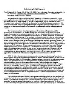
5.2.1 Direct and indirect effects, suppression and other surprises If the predictor set xi , x j are uncorrelated, then each separate variable makes a unique contribution to the dependent variable, y, and R2 ,the amount of variance accounted for in y, is the sum of the individual r2 . In that case, even though each predictor accounted for only 10% of the variance of y, with just 10 predictors, there would be no unexplained variance. Unfortunately, most predictors are correlated, and the β s found in 5.5 or 5.7 are less than the original correlations and since R2 = ∑ βi rxi y = β � rxy the R2 will not increase as much as it would if the predictors were less or not correlated. An interesting case that occurs infrequently, but is important to consider, is the case of suppression. A suppressor may not correlate with the criterion variable, but, because it does correlate with the other predictor variables, removes variance from those other predictor variables (Nickerson, 2008; Paulhus et al., 2004). This has the effect of reducing the denominator in equation 5.5 and thus increasing the betai for the other variables. Consider the case of two predictors of stock broker success: self reported need for achievement and self reported anxiety (Table 5.1). Although Need Achievement has a modest correlation with success, and Anxiety has none at all, adding Anxiety into the multiple regression increases the R2 from .09 to .12. An explanation for this particular effect might be that people wo want to be stock brokers are more likely to say that they have high Need Achievement. Some of this variance is probably legitimate, but some might be due to a tendency to fake positive aspects. Low anxious scores could reflect a tendency to fake positive by denying negative aspects. But those who are willing to report being anxious probably are anxious, and are telling the truth. Thus, adding anxiety into the regression removes some misrepresentation from the Need Achievement scores, and increases the multiple R1

5.2.2 Interactions and product terms: the need to center the data In psychometric applications, the main use of regression is in predicting a single criterion variable in terms of the linear sums of a predictor set. Sometimes, however, a more appropriate model is to consider that some of the variables have multiplicative effects (i.e., interact) such the effect of x on y depends upon a third variable z. This can be examined by using the product terms of x and z. But to do so and to avoid problems of interpretation, it is first necessary to zero center the predictors so that the product terms are not correlated with the additive terms. The default values of the scale function will center as well as standardize the scores. To just center a variable, x, use scale(x,scale=FALSE). This will preserve the units of x. scale returns a matrix but the lm function requires a data.frame as input. Thus, it is necessary to convert the output of scale back into a data.frame. A detailed discussion of how to analyze and then plot data showing interactions between experimental variables and subject variables (e.g., manipulated positive affect and extraversion) or interactions of subject variables with each other (e.g., neuroticism and extraversion) 1

Atlhough the correlation values are enhanced to show the effect, this particular example was observed in a high stakes employment testing situation.

5.2 Multiple regression

131

Table 5.1 An example of suppression is found when predicting stockbroker success from self report measures of need for achievement and anxiety. By having a suppressor variable, anxiety, the multiple R goes from .3 to .35. > stock > mat.regress(stock,c(1,2),3) Nach Anxiety Success achievement 1.0 -0.5 0.3 Anxiety -0.5 1.0 0.0 Success 0.3 0.0 1.0 $beta Nach Anxiety 0.4 0.2 $R Success 0.35 $R2 Success 0.12

Independent Predictors

Correlated Predictors

rx1y

rx1y

X1

X1 ß 1 x y

ß 1 x y rx1x2

Y

Y

ßx2y

ßx2y

X2

X2 rx2y

rx2y

Suppression

Missing variable rx1y

rx1y

X1

X1 ß 1 x y

rx1x2

ßx2y

ß Y

zx1 ß

z ß

X2

Y

zy

zx2 X2 rx2y

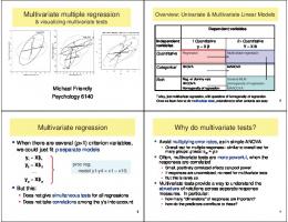
Fig. 5.1 There are least four basic regression cases: The independent predictor where the βi are the same as the correlations; the normal, correlated predictor case, where the βi are found as in 5.7; the case of suppression, where although a variable does not correlate with the criterion, because it does correlate with a predictor, it will have useful βi weight; and the case where the model is misspecified and in fact a missing variable accounts for the correlations.

132

5 Multiple correlation and multiple regression

is beyond the scope of this text and is considered in great detail by Aiken and West (1991) and Cohen et al. (2003), and in less detail in an online appendix to a chapter on experimental approaches to personality Revelle (2007), http://personality-project.org/r/ simulating-personality.html. In that appendix, simulated data are created to show additive and interactive effects. An example analysis examines the effect of Extraversion and a movie induced mood on positive affect. The regression is done using the lm function on the centered data (Table 5.2). The graphic display shows two regression lines, one for the simulated “positive mood induction”, the other for a neutral induction. Table 5.2 Linear model analysis of simulated data showing an interaction between the personality dimension of extraversion and a movie based mood induction. Adapted from Revelle (2007). > # a great deal of code to simulate the data > mod1 print(summary(mod1,digits=2) Call: lm(formula = PosAffect ~ extraversion * reward, data = centered.affect.data) Residuals: Min 1Q Median -2.062 -0.464 0.083

3Q 0.445

Max 2.044

Coefficients: Estimate Std. Error t value Pr(>|t|) (Intercept) -0.8401 0.0957 -8.8 6e-14 *** extraversion -0.0053 0.0935 -0.1 0.95 reward1 1.6894 0.1354 12.5 partial.r(R.mat,c(1:3),c(4:5)) #specify the matrix for input, and

the columns for the X and Z variables

V1 V2 V3 V1 1.00 0.46 0.38 V2 0.46 1.00 0.32 V3 0.38 0.32 1.00

The semi-partial correlation, also known as the part-correlation is the correlation between xi and y removing the effect of the other x j from the predictor, xi , but not from the criterion, y. It is just rxi y − rxi x j rx j y (5.11) r(xi .x j )(y) = � (1 − rx2i x j )

express form

136

in

5 Multiple correlation and multiple regression

matrix

5.3.1 Alternative interpretations of the partial correlation Partial correlations are used when arguing that the effect of xi on y either does or does remain when other variables, x j are statistically “controlled”. That is, in Table 5.3, the correlation between V1 and V2 is very high, even when the effects of V4 and V5 are removed. But this interpretation requires that each variable is measured without error. An alternative model that corrects for error of measurement (unreliability) would show that when the error free parts of V4 and V5 are used as covariates, the partial correlation between V1 and V2 becomes 0.. This issue will be discussed in much more detail when considering models of reliability as well as factor analysis and structural equation modeling.

5.4 Alternative regression techniques That the linear model can be used with categorical predictors has already been discussed. Generalizations of the linear model to outcomes than are not normally distributed fall under the class of the generalized linear model and can found using the glm function. One of the most common extensions is to the case of dichotomous outcomes (pass or fail, survive or die) which may be predicted using logistic regression. Another generalization is to non-normally distributed count data or rate data where either Poisson regression or negative binomial regression are used. These models are solved by iterative maximum likelihood procedures rather than ordinary least squares as used in the linear model. The need for these generalizations is that the normal theory of the linear model is inappropriate for such dependent variables. (e.g., what is the meaning of a predicted probability higher than 1 or less than 0?) The various generalizations of the linear model transform the dependent variable in some way so as to make linear changes in the predictors lead to linear changes in the transformed dependent variable. For more complete discussions of when to apply the linear model versus generalizations of these models, consult Cohen et al. (2003) or Gardner et al. (1995).

5.4.1 Logistic regression Consider, for example, the case of a binary outcome variable. Because the observed values can only be 0 or 1, it is necessary to predict the probability of the score rather than the score itself. But even so, probabilities are bounded (0,1) so regression estimates less than 0 or greater than 1 are meaningless. A solution is to analyze not the data themselves, but rather a monotonic transformation of the probabilities, the logistic function: p(Y |X) =

1 1 + e−(β0 +β x)

.

5.4 Alternative regression techniques

137

Using deviation scores, if the likelihood, p(y), of observing some binary outcome, y, is a continuous function of a predictor set, X, where each column of X, xi , is related to the outcome probability with a logistic function where β0 is the predicted intercept and βi is the effect of xi 1 p(y|x1 . . . xi . . . xn ) = 1 + e−(β0 +β1 x1 +...βi xi +...βn xn ) and therefore, the likelihood of not observing y, p(y), ˜ given the same predictor set is p(y|x ˜ 1 . . . xi . . . xn ) = 1 −

1 1 + e−(β0 +β1 x1 +...βi xi +...βn xn )

=

e−(β0 +β1 x1 +...βi xi +...βn xn ) 1 + e−(β0 +β1 x1 +...βi xi +...βn xn )

then the odds ratio of observing y to not observing y is p(y|x1 . . . xi . . . xn ) 1 = −(β +β x +...β x +...β x ) = e(β0 +β1 x1 +...βi xi +...βn xn ) . n n i i 0 1 1 p(y|x ˜ 1 . . . xi . . . xn ) e Thus, the logarithm of the odds ratio (the log odds) is a linear function of the xi : ln(odds) = β0 + β1 x1 + . . . βi xi + . . . βn xn = β0 + β X

(5.12)

Consider the probability of being a college graduate given the predictors of age and several measures of ability. The data set sat.act has a measure of education (0 = not yet finished high school, ..., 5 have a graduate degree). Converting this to a dichotomous score (education >3) to identify those who have finished college or not, and then predicting this variable by a logistic regression using the glm function shows that age is positively related to the probability of being a college graduate (not an overly surprising result) as is a higher ACT (American College Testing program) score. The results are expressed as changes in the logarithm of the odds for unit changes in the predictors. Expressing these as odds ratios may be done by taking the anti-log (i.e., the exponential) of the parameters. The confidence intervals of the parameters or of the Odds Ratios may be found by using the confinit function (Table 5.4).

5.4.2 Poisson regression, quasi-Poisson regression, and negative-binomial regression If the underlying process is thought to be binary with a low probability of one of the two alternatives (e.g., scoring a goal in a football tournament, speaking versus not speaking in a classroom, becoming sick or not, missing school for a day, dying from being kicked by a horse, a flying bomb hit in a particular area, a phone trunk line being in use, etc.) sampled over a number of trials and the measure is the discrete counts (e.g., 0, 1, ... n= number of responses) of the less likely alternative, one appropriate distributional model is the Poisson. The Poisson is the limiting case of a binomial over N trials with probability p for small p. For a random variable, Y, the probability that it takes on a particular value, y, is p(Y = y) =

e−λ λ y y!

where both the expectation (mean) and variance of Y are

138 Table 5.4 parameters odds ratios intervals of > > > > >

5 Multiple correlation and multiple regression An example of logistic regression using the glm function. The resulting coefficients are the of the logistic model expressed in the logarithm of the odds. They may be converted to by taking the exponential of the parameters. The same may be done with the confidence the parameters and of the odds ratios.

data(sat.act) college 3) +0 #convert to a binary variable College data(epil) > summary(glm(y~trt+base,data=epil,family=poisson)) Call: glm(formula = y ~ trt + base, family = poisson, data = epil) Deviance Residuals: Min 1Q Median -4.6157 -1.5080 -0.4681

3Q 0.4374

Max 12.4054

Coefficients: Estimate Std. Error z value Pr(>|z|) (Intercept) 1.278079 0.040709 31.396 < 2e-16 *** trtprogabide -0.223093 0.046309 -4.817 1.45e-06 *** base 0.021754 0.000482 45.130 < 2e-16 *** --Signif. codes: 0 ^ O***~ O 0.001 ^ O**~ O 0.01 ^ O*~ O 0.05 ^ O.~ O 0.1 ^ O ~ O 1 (Dispersion parameter for poisson family taken to be 1) Null deviance: 2517.83 Residual deviance: 987.27 AIC: 1759.2

on 235 on 233

degrees of freedom degrees of freedom

Number of Fisher Scoring iterations: 5 > summary(lm(y~trt+base,data=epil)) lm(formula = y ~ trt + base, data = epil) Residuals: Min 1Q -19.40019 -3.29228

Median 0.02348

3Q 2.11521

Max 58.88226

Coefficients: Estimate Std. Error t value Pr(>|t|) (Intercept) -2.27396 0.96814 -2.349 0.0197 * trtprogabide -0.91233 1.04514 -0.873 0.3836 base 0.35258 0.01958 18.003 > > > > > > > > > > >

set.seed(42) nt = 4 time