foundry, which produces iron castings and uses hand molding machines. A mathematical ... rial/Enterprise Resource Planning) related tools. It is a common ...
Multiple criteria lot-sizing in a foundry using evolutionary algorithms Jerzy Duda, Andrzej Osyczka AGH University of Science and Technology, Faculty of Management, Dept. of Applied Computer Science, ul. Gramatyka 10, 30-067 Kraków, Poland {JDuda,AOsyczka}@zarz.agh.edu.pl
Abstract. The paper describes the application of multiobjective evolutionary algorithms in multicriteria optimization of operational production plans in a foundry, which produces iron castings and uses hand molding machines. A mathematical model that maximizes utilization of the bottleneck machines and minimizes backlogged production is presented. The model includes all the constraints resulting from the limited capacities of furnaces and machine lines, limited resources, customers requirements and the requirements of the manufacturing process itself. Test problems based on real production data were used for evaluation of the different evolutionary algorithm variants. Finally, the plans were calculated for a nine week rolling planning horizon and compared to real historical data.
1 Introduction One of the authors has been working for a Polish foundry to develop the software which would help to improve shop production planning process. A weekly task for the planners at the operational level is to say how many castings for which orders will be produced on molding machines during all working shifts. The planning process is done manually with a little support of spreadsheets and basic MRPII/ERP (Material/Enterprise Resource Planning) related tools. It is a common practice not only in this particular foundry. The survey conducted by Van Voorhis and Peters [10] has shown that also in the USA only a few foundries used specialized software to assist the planning and scheduling process while the majority of them did it manually. The production in small and medium iron foundries is often done in short series so the planners must take into consideration many orders, each for a different product. In the considered foundry there were about 100–200 active orders a week for 10 to 500 castings of various weight and iron grade. The castings manufacturing process itself can be divided into following steps: designing a pattern, preparing molding sand and cores, making molds, melting and pouring hot iron and finally finishing operations. The patterns are prepared in a separated pattern shop and once they are made they can be used many times. If a casting requires cores, they are made in a core shop. Cores usually can be prepared earlier, even a few days before they are put in a mold. Next molding sand is compacted
around a pattern in a flask thus creating a mold. Then hot iron, melted in electric furnaces is poured into the flasks, which are left to solidify. After several hours the castings are taken from the molds and they undergo cleaning and finishing operations in a dressing shop. Operations for the pattern shop are planned independently of the main production process. Operations for the core shop and the dressing shop can be planned easily on the basis of a molding plan unless the plan includes an enormous number of castings which require many cores or a lot of time to be finished. This situation is very rare in the foundry so it will not be considered in the optimization model. Thus a priority for the planners is to prepare an appropriate molding plan connected with a pouring schedule for the furnaces. These plans must be coordinated as melted iron cannot wait too long to be poured, and also the room for the molds waiting for pouring is limited. While building the plan many technological and organizational constraints have to be taken into consideration. The most significant are: − capacities of furnaces and molding machines, − the number, desired delivery date and cast iron grade of ordered castings, − the number of different castings which can be produced during one shift (setup times are included in forming times), − the number of flasks of various size available during a working shift, − the minimum batch size a customer can accept. The data for the optimization model can be collected nearly automatically from the existing production control system.
2 Mathematical model A mathematical model was formulated on the basis of the classical discrete capacitated lot-sizing problem with single level and multi item production on parallel machines. A similar approach can be found in Santos-Mezo et al. paper [8], which discusses a lot-sizing problem in an automated foundry. The model proposed in this paper, however differs in two main points. A commonly used minimization of an artificially built sum cost function has been replaced by two objective functions indicated directly by the planners. Another modification is that the equality constraint balancing inventory and demand has been changed into an inequality constraint. The following symbols are used: Decision variables: xijtz – number of castings planned for order i to be manufactured on machine j during day t and shift z, vhtz – number of heats of grade h during day t and shift z. Data: τ – week for which the plan is created, k – number of working days in a week, mj – number of working shifts for machines type j, nj – number of active orders for machines type j, CP – daily melting capacity of the furnaces [kg],
W – weight of single heat [kg], CFj – capacity of molding machines type j during a working shift [minutes], wij – total iron weight needed to produce single i casting [kg], aij – time of making a mold for casting i on machine j [minutes], dij – ordered number of castings of type i to be produced on machine j, γ – number of iron grades, gij – iron grade for casting i, gij∈{1,...,γ}, ω – number of flask types, So – flask number of type o available during a working shift, qij – flask type in which a mold for casting i is prepared, qij∈{1,...,ω}, κj – number of different castings which can be produced on machine type j during one working shift, δij – due week for castings of type i to be produced on machine j, πti j – penalty value for tardiness, πei j – penalty value for earliness. First objective function: nj
l
mj
k
maximize ∑ ∑ ∑ ∑ ( j =1 i =1 t =1 z =1
x ijtz wij kC P
+
x ijtz a ij km j C Fj
(1) )
Second objective function: l
nj
k
mj
k
mj
minimize ∑ ∑ ((d ij − ∑ ∑ x ijtz )(τ − δ ij )π tij (τ > δ ij )(d ij > ∑ ∑ x ijtz )) j =1 i =1
t =1 z =1
l
(2)
t =1 z =1
nj
mj
k
+ ∑ ∑ ((d ij − ∑ ∑ x ijtz )(τ − δ ij )π ije (τ < δ ij )) j =1 i =1
t =1 z =1
Constraints: γ
∑ v hzt W ≤ C P ,
t = 1,..., k ,
h =1
nj
∑ xijtz a ij i =1
k
≤ C Fj ,
j = 1,..., l , t = 1,..., k ,
mj
∑ ∑ xijtz ≤ dij , nj
∑∑ ( xijtz wij ( gij = h)) ≤ vhtzW , j =1 i =1
nj
∑ ( xijtz i =1
l
nj
> 0) ≤ κ j ,
∑ ∑ ( xijtz (qij = o)) ≤ So , j =1 i =1
z = 1,..., m j
h = 1,..., γ , t = 1,..., k , z = 1,..., m j
j = 1,..., l , t = 1,..., k ,
z = 1,..., m j
o = 1,..., ω , t = 1,..., k ,
(4)
(5)
j = 1,..., l , i = 1,..., n j
t =1 z =1
l
(3)
z = 1,..., m j
z = 1,..., m j
(6)
(7)
(8)
The first objective function (1) maximizes the utilization of both furnaces and molding machines as these are bottlenecks in the production system. Although the function (1) is to be maximized, for the sake of convenience it is transformed to minimization by multiplying it by –1. The second objective function (2) minimizes the penalty for not making as many castings as ordered by the customer on time or for making them earlier than in the week agreed with the customer. Constraints (3) and (4) are the capacity constraints for the furnaces and the molding machines, respectively. Constraint (5) ensures that no more production can be planned than ordered by the customer. In the classic lot-sizing model constraint (5) is an equality. However, in the considered foundry the sum of items ordered usually exceeds production capability so backlogging is a common practice and customers receive their castings in several batches. The penalty function (2) ensures that backlogging would is kept at a possibly low level. Inequality constraint (6) limits the weight of the planned castings of a particular cast iron grade to the weight of the metal which has to be melted. According to constraint (7) no more than κj different castings may be produced during one working shift. The last constraint (8) limits the flask availability. The model is formulated as a nonlinear problem, however it is possible to change it into an integer programming formulation by entering additional binary variables.
3 Evolutionary algorithm A weekly plan for molding machines is coded in a single chromosome using integer gene values. A single gene represents quantity of castings planned for production or equals zero if the production for particular order during a given shift is not planned. This can be presented as the matrix shown in figure 1. 1st working shift
2nd working shift
mj-th working shift
x1111, x2111,..., xn1111, x1112, x2112,..., xn1112, ..., x111m1, x211m1,..., xn111m1, x1121, x2121,..., xn1121, x1122, x2122,..., xn1122, ..., x112m1, x212m1,..., xn112m1, ... x11k1, x21k1,..., xn11k1, x11k2, x21k2,..., xn11k2, ..., x11km1, x21km1,..., xn11km1,
machine 1st type
x1211, x2211,..., xn1211, x1212, x2212,..., xn1212, ..., x121m1, x221m1,..., xn121m1, x1221, x2221,..., xn1221, x1222, x2222,..., xn1222, ..., x122m1, x222m1,..., xn122m1, ... x12k1, x22k1,..., xn12k1, x12k2, x22k2,..., xn12k2, ..., x12km1, x22km1,..., xn12km1,
machines 2nd type
... x1l11, x2l11,..., xn1l11, x1l12, x2l12,..., xn1l12, ..., x1l1m1, x2l1m1,..., xn1l1m1, x1l21, x2l21,..., xn1l21, x1l22, x2l22,..., xn1l22, ..., x1l2m1, x2l2m1,..., xn1l2m1, ... x1lk1, x2lk1,..., xn1lk1, x1lk2, x2lk2,..., xn1lk2, ..., x1lkm1, x2lkm1,..., xn1l km1, Fig. 1. Molding plan coded in a chromosome
machine l-th type
This chromosome structure leads to a situation where a correct plan should have a lot of zeroes, regarding constraint (7). To avoid keeping incorrect individuals in a population a simple repair algorithm is introduced. Whenever constraint (7) is violated for one of the machines and working shifts, the smallest lots planned so far are eliminated successively from the plan until the number of different lots which are allowed for production during one working shift is reached. Note that there are no vhtz variables related to the pouring schedule in a chromosome. Instead of this a second repair algorithm is used. Its role is to keep molding plans always acceptable from a pouring schedule point of view. This means that there is enough hot iron for filling all the molds prepared. The idea of the algorithm is similar to the first repairing algorithm. If the maximum number of heats of a particular iron grade is exceeded than the lot with the minimum weight of castings is removed from the plan. A new crossover operator which operates on working shifts is introduced. Two shifts in a plan are chosen randomly. Then the lot sizes in these shifts are swapped. The crossover operator is used with the probability of 80%. A mutation pool is being created using tournament selection together with an elitist mechanism. The simple uniform mutation is chosen experimentally as a mutation operator and is used for altering genes with the probability of 0.1%. Many multicriteria evolutionary algorithms have been proposed in literature. The survey of them can be found in Coello Coello [1] or in Osyczka [7]. Among the algorithms proposed later, two are regarded as the most effective: NSGAII created by Deb et al. [2] and SPEA2 proposed by Zitzller et al. [11]. Both algorithms were used for generating the final approximation of Pareto front. Additionally, a slightly modified SPEA2 algorithm version has been tested. In the environmental selection process the best individuals regarding all the objective functions are copied into a mutation pool obligatorily. This modification will be denoted as SPEA2e (SPEA2 with extended elitism) in this paper. The statistics proposed by Fonseca and Fleming [3] in the version implemented by Knowles and Corne [5] is used to test which multicriteria evolutionary algorithm performs better in terms of the presented model and test problems. Although the statistics fails in some cases [12], it enables us to compare two Pareto front approximation sets when a reference set is not known.
4 Test problems Test sets have been chosen from the production control computer system used in the foundry described in this study. The first test problem (fixed1) consists of 84 orders while the second (fixed2) has exactly 100 orders. There are four molding lines in the considered factory, each consisting of two molding machines, one for making a cope and one for making a drag (top and bottom parts of a flask). However, there are only three types of molding machines. The type of machine which is used for making a mold for a particular casting is stated in its operation sheet. Tables 1, 2 and 3 shows detailed specification of the orders which are to be produced on machine types A, B, and C, respectively.
-3 0 0 0 0 1 2 3
0.460 2.707 2.289 0.511 0.847 1.482 0.583 0.870
forming time [min] iron grade
9 16 37.3 25.4 4 10 22 34.7 30.2 5 11 14 51.0 27.3 4 12 249 62.8 29.3 4 13 30 43.0 26.1 4 14 6 54.6 31.8 4 15 44 80.0 35.0 4 16 548 79.0 37.4 4
penalty coef.
4 4 4 4 4 4 4 4
due week
30.5 32.1 29.0 31.8 27.3 32.6 25.6 25.4
weight [kg]
61.2 82.0 61.6 54.0 43.0 65.0 48.0 30.4
order no. flasks left to make
weight [kg]
282 37 26 3 125 226 102 16
penalty coef.
flasks left to make
1 2 3 4 5 6 7 8
forming time [min] iron grade due week
order no.
Table 1. Detailed specification of fixed1 problem orders for machines type A (big flasks)
3 3 3 3 4 5 5 5
1.203 1.045 1.085 0.485 0.538 0.518 1.135 0.989
0.159 0.159 0.069 0.183 0.125 0.128 0.321 0.321 0.458 0.108 0.153 0.831 0.831 0.217 0.238 0.209 0.310 0.169 0.147 0.161 0.175 0.094
23 24 25 26 27 28 29 30 31 32 33 34 35 36 37 38 39 40 41 42 43 44
16 37 26 24 229 8 16 31 6 11 16 5 5 19 10 112 458 32 184 52 59 545
12.9 12.8 15.9 21.4 13.5 6.8 6.0 1.8 10.4 9.1 10.8 10.9 13.1 15.2 13.9 9.6 12.2 12.6 23.8 8.3 4.2 28.9
penalty coef.
-3 -3 -3 -3 -2 -2 -2 -1 0 0 0 0 0 0 0 0 0 0 0 0 0 1
due week
5 5 2 4 4 2 4 4 5 4 4 4 4 2 2 5 5 5 5 5 5 5
forming time [min] iron grade
14.2 14.2 11.8 11.6 5.5 13.9 14.2 14.2 15.3 12.7 14.3 13.9 13.9 12.1 12.1 12.6 12.0 13.9 13.9 13.9 13.9 12.3
weight [kg]
24.0 24.0 18.0 9.3 3.4 15.6 15.1 15.1 16.2 14.3 18.1 25.0 25.0 10.4 12.2 9.0 13.8 12.4 11.6 11.0 12.0 12.0
order no. flasks left to make
weight [kg]
32 35 231 424 8 31 404 538 432 44 28 83 91 212 159 4 47 16 16 16 16 133
penalty coef.
flasks left to make
1 2 3 4 5 6 7 8 9 10 11 12 13 14 15 16 17 18 19 20 21 22
forming time [min] iron grade due week
order no.
Table 2. Detailed specification of fixed1 problem orders for machines type B (small flasks)
13.2 13.2 13.2 15.1 11.5 14.3 14.3 3.6 13.9 13.9 13.9 14.0 14.0 13.1 12.3 13.3 12.7 13.0 12.1 13.0 11.5 13.2
1 1 1 1 2 3 3 3 3 3 3 3 3 3 3 3 3 3 5 5 5 5
0.096 0.126 0.117 0.207 0.423 0.083 0.078 0.093 0.161 0.133 0.158 0.030 0.049 0.183 0.055 0.072 0.212 0.209 0.348 0.370 0.138 0.431
5 5 5 5 4 5 5 5 5 5 5 5 5 2 2 5 5 5 4 5 5 4
The number of flasks to make is calculated as the number of castings ordered by the customers divided by the number of castings which fit in a single flask. Thus the weight and forming time refer to the whole flask, not to a single casting.
forming time [min]
iron grade
due week
penalty coef.
0.209 0.501 0.239 0.299 0.652 0.454 1.291 0.322 1.389 0.758 0.684 0.535
weight [kg]
-3 -3 -2 -2 -2 -1 0 0 0 0 0 1
order no.
4 4 4 4 4 4 5 4 5 5 4 4
flasks left to make
17.2 15.1 16.4 18.1 19.0 17.7 19.2 17.3 16.5 19.0 18.0 15.9
penalty coef.
15.6 18.2 10.7 10.8 52.2 29.6 70.0 18.6 62.0 29.5 23.0 18.3
due week
3 257 26 25 58 196 4 26 37 43 265 67
forming time [min] iron grade
flasks left to make
1 2 3 4 5 6 7 8 9 10 11 12
weight [kg]
order no.
Table 3. Detailed specification of fixed1 problem orders for machines type C (medium flasks)
13 14 15 16 17 18 19 20 21 22 23 24
36 36 83 122 96 249 22 62 108 27 401 53
6.9 3.4 5.8 9.0 23.6 13.6 21.7 26.8 30.2 36.6 30.4 39.2
2.9 1.4 2.4 6.8 16.7 10.2 18.6 18.4 14.1 14.7 17.4 18.6
5 5 5 5 5 5 5 4 4 4 4 4
2 2 2 3 3 3 3 5 5 5 5 5
0.203 0.099 0.171 0.122 0.148 0.181 0.279 0.186 0.499 0.248 0.489 0.391
Due week is a week which has been agreed with the customer as a term of delivery. A negative number indicates that the remaining castings are overdue. A penalty coefficient for not making castings on time is calculated on the basis of the castings price and the customer’s importance rating. A penalty value for earliness is set arbitrarily to 60% of the penalty coefficient value for tardiness, although this ratio can be set differently by the decision maker. There are 3 working shifts for the lines of machine type A and C while there are only 2 working shifts for the lines of machine type B. A common practice in the considered foundry is that only two different castings can be produced during one working shift, so κ1 and κ3 are set to 2 and κ2=4. The total daily capacity of the furnaces is 21 000 kg while a single pouring weighs 1400 kg, i.e. there are 15 heats a day. The number of flasks available for all molding machines during one working shift is limited to 50 big flasks, 100 medium and 120 small ones. The goal for the two fixed planning horizon problems is to create a set of plans for a week which consists of 5 working days. The task for rolling horizon problem, presented later in this paper, is to build a series of weekly molding plans for 9 weeks, taking into account production quantities planned for previous weeks and the new orders appearing every week. The second test set for fixed planning horizon (fixed2) and the set for the 9 week rolling horizon (rolling1) can be found at http://www.zarz.agh.edu.pl/jduda/foundry.
4 Results for a single week Evolutionary algorithms for both test problems fixed1 and fixed2 were run for 30 000 generations. The size of the population and the size of the external sets were set to 50 individuals. The number of evaluated generations and the size of the population were
chosen experimentally, as the best compromise between the solution quality and the computational time. It took about 10–15 minutes to generate a single set of plans, which is reasonable from a practical point of view. Calculations were repeated 20 times for every combination of the problem and algorithm type. Figure 2 shows nondominated sets generated using NSGAII, SPEA2 and SPEA2e algorithms for the first test problem (fixed1). A nondominated set for a given MOEA was obtained by putting all the solutions from 20 runs together and choosing only nondominated ones. The solutions in a single set, however, did not differ from the solutions in the remaining 19 sets for more than 3% regarding each objective function. 1800 1600
NSGAII
SPEA2
SPEA2e
penalty value
1400 1200 1000 800 600 400 200 1.8
1.825
1.85
1.875
1.9
1.925
1.95
1.975
2
capacity utilization
Fig. 2. Pareto sets achieved for problem fixed1
It is worth noticing that the solutions generated by the NSGAII algorithm preferred the first objective function to the second one unlike SPEA2 algorithms. In 20 runs the algorithm achieved the highest overall machine and furnace utilization, however accompanied by the biggest penalty value. Table 4 shows the area percentage of the solution space for which the tested algorithms are unbeaten by the others and the area percentage for which the tested algorithms beat all the others. Table 4. Knowles Corne statistic for fixed1 problem.
unbeaten beats all
NSGAII
SPEA2
SPEA2e
42.6 0
81.2 0.2
99.8 0.5
The calculations were done using Knowles and Corne algorithm at 0.95 confidence level with 500 lines generated. The area for which the tested algorithms remain unbeaten is the biggest for both versions of SPEA2 algorithms with a little superiority of the latter. However, SPEA2e algorithm beats all its rivals only in 0.5% of the solution space. Figure 3 illustrates the Pareto sets generated for fixed2 problem. The NSGAII algorithm again gave the highest utilization level, thus confirmed its tendency to prefer the first objective function. This time the SPEA2 algorithm seems to prefer the second objective function to the first one. Only the SPEA2e treats both optimization criteria equally in this case. Nevertheless, these observations cannot be generalized to other problems without making additional tests and the use of additional metrics like for example generalization distance and error ratio proposed by Van Veldhuizen and Lamont [9]. 1600 1400
NSGAII
SPEA2
SPEA2e
penalty value
1200 1000 800 600 400 200 0 1.8
1.825
1.85
1.875
1.9
1.925
1.95
1.975
2
capacity utilization
Fig. 3. Pareto sets achieved for problem fixed2
Fonseca and Fleming statistics, presented in Table 5, indicates that SPEA2e algorithm in the case of fixed2 problem is unbeaten by the other algorithms, but there is no solution space where any of the algorithms beats the others. Table 5. Knowles Corne statistic for fixed1 problem.
unbeaten beats all
NSGAII
SPEA2
SPEA2e
54.7 0
81.2 0
100 0
The general conclusion is that all the tested multicriteria evolutionary algorithms perform well enough to be applicable in real-world production optimization. The
choice of the algorithm will be easier if the planner regards one objective function a little more important that the other. To build the series of weekly plans for the rolling horizon problem (rolling1) the proposed modification of SPEA2 algorithm was chosen as it performed slightly better than the other algorithms.
6 Results for a rolling planning horizon In order to verify the effects resulting from the application of the proposed method the historical production data were compared against the plans created by the multicriteria evolutionary algorithm. The plans were build week after week within 9 weeks. Starting from 53 orders for machine type A, 129 orders for machine type B and 73 orders for machine types C (total 255 orders, at least 30% of them were overdue) in each following week new orders appeared (in the number of 3 to 21). Each time the multicriteria evolutionary algorithm delivered weekly plans, only one was automatically chosen as the accepted production plan. After choosing a single plan the remaining orders were consequently altered by the planned production quantities. Two variants of such automatic choice were considered. In the first variant a compromise solution in a min-max sense as defined by Osyczka [6] was taken. Instead of using a relative increment of objective functions, scalarized increment (9) was used, as the objective functions have very different value ranges. f ' i ( x) =
f i ( x) − f i min
(9)
f i max − f i min
In the second variant of the simulation the solution with the first objective function equaled at least 1.95 with the smallest possible value of the second objective function was taken as the plan accepted for the next week. If such solution did not exist in the obtained Pareto set, the solution with the highest utilization value was taken. Table 6 shows the utilization level of the furnaces and molding machines calculated on the basis of the historical data and compared to the utilization attained in the simulation variants. Table 6. Comparison between the results obtained in the simulation and the historical data historical average furnaces utilization (weekly) lowest furnaces utilization average molding machines utilization lowest molding machines utilization average penalty value for tardiness average penalty value for earliness
84% 77% 70% 64% 1880 230
MOEA variant 1
90% 80% 84% 73% 1610 390
MOEA variant 2
93% 82% 83% 78% 1790 410
In the first variant the average utilization level of the furnaces equaled 90%, compared to 84%, which was observed in reality. In the second variant this utilization was even higher and equaled on average 93%, but the penalty value was bigger than the one calculated on the basis of historical data. Also the average utilization level of molding machines was 1% worse than in the first variant. In the plans obtained by evolutionary algorithm this utilization equaled 85% while in reality it was only 70%. It can be seen that in case of the simulation, the overdue production generally decreased. The biggest penalty value for the production which was made earlier than required by the customers as compared with the historical data might be seen as a disadvantage. However, this was not caused by increasing the penalty value for the overdue castings, which simply means that the time from order acceptance to its realization can be shortened. In Table 7 the mini-max optimal solution obtained for the first week is shown. This solution may be viewed as the best compromise solution considering both criteria as equally important. The value of the first objective function (summarized utilization) is 1.91 (0.96 for furnaces and 0.95 for molding shop) while the value of the second objective function (summarized penalty) is 440 (373 for tardiness and 67 for earliness). Table 7. The exemplary solution obtained for the first week (order | quantity).
day/shift 1/1 1/2 1/3 2/1 2/2 2/3 3/1 3/2 3/3 4/1 4/2 4/3 5/1 5/2 5/3
machine type A 3|19 36|20 6|32 23|15 4|20 12|29 11|36 18|3 3|14 22|25 11|27 29|9 7|15 8|27 14|17 17|20 3|18 36|20 8|27 16|19 2|16 21|14 8|27 19|17 5|13 18|24 16|22 19|25 13|22 16|28
machine type B 17|98 52|134 4|56 24|137 55|157 15|118 17|133 1|140 34|93 1|94 4|98 15|85
machine type C 13|82 63|10 17|37 29|40 3|36 20|42 88|64 10|98 13|54 69|104 13|52 38|25 25|39 28|36 45|96 7|101 9|101 46|65 8|96 12|61 31|68 44|132 5|35 40|40 16|106 16|31 35|41 15|68 21|5 53|144 17|78 110|151 18|60 36|20 13|72 43|18
7. Conclusions The results presented here look very promising for the future application not only in the foundry considered, but also in other similar manufactures. The model shown in this paper will be successively complemented with new technological and organiza-
tional constraints, especially resulting from the sequence of heats. Unfortunately, reliable data concerning the costs of iron grade changes were hard to collect because they were not present in the current computer system. The multicriteria evolutionary algorithms together with the proposed repair algorithms prove to be a very effective optimization tool not only for standard test problems but also for real scale production optimization tasks. It is worth underlining that the simulation performed for a nine week rolling horizon can involve in a single run as many as 3125 variables and 345 constraints. The introduction of additional objective functions also seems to be a very interesting alternative to the traditional approach with one objective function which optimizes usually artificially constructed sum of the production and relevant costs. This paper covered only two important aspects of operational production planning: how to maintain high utilization level of bottleneck machines and how to keep backlogged production as low as possible. The two objectives analyzed in this paper are very similar to the first two criteria proposed by Gravel et al. [4] for scheduling continuous casting of aluminum. This similarity, however not intentional, confirms that the proposed approach can be applied to a wider range of planning and scheduling problems in cast making companies of various kinds. The main aim of the presented approach was to give the decision maker not a single plan which has to be implemented, but a set of plans from which she or he may choose the one which suits the best the current economical circumstances of the enterprise. The multicriteria evolutionary algorithms enable to obtain a wide spread of the solutions in a single run. This lets the decision maker to perform a quick what-if analysis before making the right planning decision. Acknowledgments This study was supported by the State Committee for Scientific Research (KBN) under Grant No. 0224 H02 2004 27 and PB 0808 T07 2003 25.
References 1. Coello Coello, C.A, Van Veldhuizen, D.A., Lamont, G.B., Evolutionary Algorithms for Solving Multi-Objective Problems, Kluwer Academic Publishers, New York (2002) 2. Deb, K., Agrawal, S., Pratab, A., Meyarivan T.: A Fast Elitist Non-Dominated Sorting Genetic Algorithm for Multi-Objective Optimization: NSGA-II. KanGAL report 200001, Indian Institute of Technology, Kanpur (2000) 3. Fonseca, C. M., Fleming, P.J., An Overview of Evolutionary Algorithms in Multiobjective Optimization. Evolutionary Computation, Vol. 3, 1 (1995) 1–16 4. Gravel M., Price, W.L., Gagné, C.: Scheduling continuous casting of aluminium using a multiple-objective ant colony optimization metaheuristic, European Journal of Operational Research, Vol. 143, 1 (2002) 218–229 5. Knowles, J.D., Corne, D.W.: Approximating the Nondominated Front using the Pareto Archived Evolution Strategy. Evolutionary Computation, Vol. 8, 2 (2000) 149–172
6. Osyczka, A.: Multicriterion Optimization in Engineering with Fortran Programs, John Wiley and Sons, New York (1984) 7. Osyczka A.: Evolutionary Algorithms for Single and Multicriteria Design Optimization, Physica Verlag, Heidelberg, New York (2002) 8. dos Santos-Meza, E., dos Santos, M.O., Arenales, M.N.: A Lot-Sizing Problem in An Automated Foundry. European Journal of Operational Research, Vol. 139, 3 (2002) 490–500 9. Van Veldhuizen, D.A., Lamont, G.B., Multiobjective Evolutionary Algorithm Research: A History and Analysis, Technical Report TR-98-03, Department of Electrical and Computer Engineering, Graduate School of Engineering, Air Force Institute of Technology, WrightPatterson AFB, Ohio (1998) 10. Voorhis, T.V., Peters F., Johnson D.: Developing Software for Generating Pouring Schedules for Steel Foundries. Computers and Industrial Engineering, Vol. 39, 3 (2001) 219–234 11. Zitzler, E., Laumanns, M., Thiele, L.: SPEA2: Improving the Strength Pareto Evolutionary Algorithm. Technical Report 103, Computer Engineering and Networks Laboratory (TIK), Swiss Federal Institute of Technology (ETH), Zurich (2001) 12. Zitzler, E., Thiele, L., Laumanns, M., Fonseca, C.M., Grunert da Fonseca, V.: Performance Assessment of Multiobjective Optimizers: An Analysis and Review. IEEE Transactions on Evolutionary Computation, Vol. 7, 2 (2003) 117–132