Multiple Hypothesis Tracking with Multiframe Assignment Using ...

14th International Conference on Information Fusion Chicago, Illinois, USA, July 5-8, 2011

Multiple Hypothesis Tracking with Multiframe Assignment Using Range and Range-rate Measurements T. Sathyan

S. Arulampalam

M. Mallick

ICT Center CSIRO Marsfield, NSW, Australia. [email protected]

Maritime Operations Division DSTO Edinburgh, SA, Australia. [email protected]

Propagation Research Associates, Inc. Marietta, GA, USA. [email protected]

Abstract—In this paper we consider the problem of multitarget tracking using range and range-rate measurements collected from a single maneuvering platform. Although bearings-only tracking has been studied extensively, only a few studies exist in the literature that consider range-only tracking. The motivating application for this work is maritime surveillance using radars equipped with inverse synthetic aperture radar mode. We consider a realistic scenario that consists of an unknown number of targets with measurement origin uncertainty due to their presence and false alarms, and imperfect radar measurements. The algorithm that we proposed is a multiple hypothesis tracker based on the multiframe assignment algorithm. Different track initialization techniques depending on whether or not initial bearing measurements are available are considered and an angleparameterized filter is used to track the targets. Simulations conducted show the effectiveness of the proposed algorithm in terms of tracking accuracy and track maintenance capability. Keywords: Multitarget tracking, multiple hypothesis tracking (MHT), data association, multiframe assignment (MFA), range and range-rate measurements, inverse synthetic aperture radar (ISAR).

I. I NTRODUCTION We study the problem of multitarget tracking using range and range-rate measurements collected by a single maneuvering platform, where the objective is to estimate the kinematic parameters, such as position and velocity, of an unknown number of targets present in the surveillance region. This problem arises for example, in maritime surveillance, where radars that can operate in the inverse synthetic aperture radar (ISAR) mode will collect high-resolution range profiles, and the information contained in these range profiles is expressed in the form of range and range-rate measurements. Although bearings-only tracking has been studied extensively in the past [1] [8] [11] [13], one can only find a very limited number of publications that study the problem of range-only tracking. In [16] conditions for target observability using range-only measurements is studied and the conclusion is that the own-ship must out-maneuver the target to achieve observability. For example, if the target is moving with a constant velocity then the own-ship must accelerate to observe the target. Filtering algorithms using range and range-range measurements are studied in [14]. In particular, for a target moving with a deterministic constant velocity trajectory, the

978-0-9824438-3-5 ©2011 ISIF

performance of the maximum likelihood estimator, an angleparameterized extended Kalman Filter (AP-EKF), and the regularized particle filter are evaluated and compared against the the Cram´er-Rao lower bound. In [5], range and range-rate measurements collected at multiple platforms are used for multitarget tracking. Using a variation of the expectation-maximization algorithm, the data association problem is solved probabilistically and the computational complexity is greatly reduced. The formulation, however, is similar to the probabilistic multiple hypothesis tracker (PMHT) and relaxes the one-to-one constraint between tracks and measurements. Although extensively studied, PMHT-type algorithms have not been shown to be superior to the traditional formulations of probabilistic data association [2] and multiple hypothesis tracking (MHT) [12], [9], both of which correctly assume that a target generates at most one measurement in every scan. In this paper we consider the problem of multitarget tracking using range and range-rate measurements in the presence of false alarms and non-unity probability of detection of the sensor. The measurements are collected by a single maneuvering platform and we assume that the number of targets is unknown. We develop an MHT algorithm that is based on the multiframe assignment (MFA). We consider two different scenarios for track initialization; with and without coarse initial bearing measurements. This is because certain types of radars such as the multi-mode Ingara radar considered in [14] can provide initial bearing measurements in what is called a scan mode, before switching to ISAR mode where only range profiles are generated. One of the conclusions of [14] is that the AP-EKF is the preferred filter for the filtering problem using range and range-rate measurements, since it provided satisfactory state estimation accuracy at modest computational cost and is robust against initialization inaccuracies. Based on this conclusion, we choose an angle-parameterized unscented Kalman filter (AP-UKF) as the state estimator in the proposed algorithm. The important issue of data association is addressed using the MFA algorithm, which formulates the data association as a discrete optimization problem. The MFA is often implemented as a sliding window and mimics the MHT within this window. Although initially developed for measurement-to-measurement

2126

association, it has been successfully applied for track-tomeasurement association as well. The rest of this paper is organized as follows. Section II describes the details of the filtering problem using range and range-rate measurements. Various aspects of the proposed algorithm are discussed in Section III, and the simulation results that illustrate the performance of the proposed algorithm are presented in Section IV. Concluding remarks are given in Section V. II. P ROBLEM D ESCRIPTION We study the problem of multitarget tracking using range and range-rate measurements in the two-dimensional plane where the targets are assumed to follow a nearly constant velocity (NCV) motion. The number of targets in the surveillance region is unknown and it is required to estimate the kinematic parameters (position and velocity) of all the targets. Assume that x𝑖𝑘 = [𝑥𝑖𝑘 , 𝑥˙ 𝑖𝑘 , 𝑦𝑖𝑘 , 𝑦˙ 𝑖𝑘 ]𝑇 denotes the state vector of target 𝑖 at scan 𝑘 (corresponding to time 𝑡𝑘 ), where (𝑥𝑖𝑘 , 𝑦𝑖𝑘 ) and (𝑥˙ 𝑖𝑘 , 𝑦˙ 𝑖𝑘 ) are the position and velocity components of the target in the Cartesian coordinates. Similarly the state of the observer is defined as x𝑜𝑘 = [𝑥𝑜𝑘 , 𝑥˙ 𝑜𝑘 , 𝑦𝑜𝑘 , 𝑦˙ 𝑜𝑘 ]𝑇 and is assumed to be deterministic and known for all values of 𝑘. A relative state vector for target 𝑖 is defined as x𝑟𝑖𝑘 = x𝑖𝑘 − x𝑜𝑘

(1)

The evolution of the relative state vector can be captured in the following dynamic equation x𝑟𝑖𝑘 = F𝑘,𝑘−1 x𝑟𝑖𝑘−1 + 𝝂 𝑖𝑘−1 − U𝑘,𝑘−1

(2)

where F𝑘,𝑘−1 is the state transition matrix, 𝝂 𝑖𝑘−1 is a zeromean white Gaussian process noise sequence with covariance matrix Q𝑖𝑘−1 that models gentle maneuvers of the target, and U𝑘,𝑘−1 is a deterministic control input that accounts for the acceleration of the observer. F𝑘,𝑘−1 and Q𝑖𝑘 are given by ] [ 1 𝜏𝑘 (3) F𝑘,𝑘−1 = I2 ⊗ 0 1 ] [ 3 𝜏𝑘 /3 𝜏𝑘2 /2 Q𝑖𝑘 = I2 ⊗ 𝑞˜𝑖 (4) 𝜏𝑘 𝜏𝑘2 /2 where 𝜏𝑘 = 𝑡𝑘 − 𝑡𝑘−1 , 𝑞˜𝑖 is the power spectral density of the noise sequence 𝝂 𝑖𝑘 , I2 is a 2 × 2 identity matrix, and ⊗ denotes the Kronecker product. U𝑘,𝑘−1 is given by ⎡ ⎤ 𝑥𝑜𝑘 − 𝑥𝑜𝑘−1 − 𝜏𝑘 𝑥˙ 𝑜𝑘−1 ⎢ ⎥ 𝑥˙ 𝑜𝑘 − 𝑥˙ 𝑜𝑘−1 ⎥ U𝑘,𝑘−1 = ⎢ (5) ⎣ 𝑦𝑜𝑘 − 𝑦𝑜𝑘−1 − 𝜏𝑘 𝑦˙ 𝑜𝑘−1 ⎦ 𝑦˙ 𝑜𝑘 − 𝑦˙ 𝑜𝑘−1 The radar measures the range and range-rate of the targets it detects with a non-unity probability of detection 𝑃𝐷 . The radar can also generate false measurements, the number of which is assumed to be Poisson distributed with density 𝜆 and they are assumed to be distributed uniformly in the measurement space. The 𝑗th measurement at scan 𝑘 is then given by ⎧ [ ] ℎ𝑟 (x𝑟𝑘 ) ⎨ + v𝑗𝑘 if target originated 𝑟 ℎ𝑟˙ (x𝑘 ) (6) z 𝑗𝑘 = ⎩ ˜ z if false alarm

where the range and range-rate measurement functions ℎ𝑟 (x𝑟𝑘 ) and ℎ𝑟˙ (x𝑟𝑘 ) are given by √ ℎ𝑟 (x𝑟𝑘 ) = (𝑥𝑟𝑘 )2 + (𝑦𝑘𝑟 )2 (7) and 𝑥𝑟 𝑥˙ 𝑟 + 𝑦𝑘𝑟 𝑦˙ 𝑘𝑟 ℎ𝑟˙ (x𝑟𝑘 ) = √ 𝑘 𝑟𝑘 (𝑥𝑘 )2 + (𝑦𝑘𝑟 )2

(8)

respectively. The measurement noise v𝑗𝑘 is assumed to be Gaussian distributed with zero-mean and covariance matrix 𝑅 = diag(𝜎𝑟2 , 𝜎𝑟2˙ ), that is v𝑘,𝑗 ∼ 𝒩 (v𝑘,𝑗 ; 0, 𝑅), where 𝜎𝑟 and 𝜎𝑟˙ , respectively, are the range and range-rate measure˜ is a two-dimensional vector ment error standard deviations. z consisting of the values of range and range-rate corresponding to the false alarm. Note that a target index is not used in the measurement equation since it is not known to the tracker. Let the number of measurements reported by the radar at scan 𝑘 be 𝑀𝑘 and the number of targets in surveillance 𝑘 region be 𝑁𝑘 . Also let 𝑍𝑘 = {z𝑗𝑘 }𝑀 𝑗𝑘 =1 summarize all the measurements received at scan 𝑘. The objective now is to estimate the states of all targets in the surveillance region using the measurements 𝑍𝑘 , 𝑘 = 1, 2, . . . reported by the radar. III. P ROPOSED A LGORITHM The proposed algorithm initializes a track for each measurement received in the very first scan. Subsequent scans of measurements are associated with the tracks using the MFA algorithm, and a track is updated with the measurement that is assigned to it. New tracks are initialized from every unassigned measurement. We consider track initialization with and without initial bearing measurement, since in certain applications knowledge about the initial bearing to the target is made available to the tracker. For example, in the Ingara multi-mode radar considered in [14], during the very first scan the radar is in scan mode and generates coarse bearing measurements along with range and range-rate measurements. After this initial scan, it switches to the ISAR mode where it generates highresolution range profiles, without any bearing information. Availability of the initial bearing information, however, is not mandatory for the operation of the proposed algorithm. State estimation using range and range-rate measurements is essentially a nonlinear estimation problem and hence, requires a nonlinear filtering algorithm. If precise initial bearing information is available to initialize the tracks, then a standard extended Kalman filter (EKF) is adequate for the state estimation. For scenarios where the initial bearing information is coarse or unavailable, [14] developed an AP-EKF, which resembles the range-parameterized EKF proposed for bearingsonly tracking, and it was shown that the AP-EKF is more robust against initialization errors that the standard EKF. In this paper we replace the EKF with an unscented Kalman filter (UKF) and use angle-parameterization. The UKF is preferred over EKF since it provides a better approximation to the nonlinear filtering problem compared to the standard EKF. Further, unlike the EKF, the UKF does not require the

2127

evaluation of the Jacobian or the Hessian of the nonlinear state function, and as a result it is easier to implement. Details of various aspects of the proposed algorithm – angle-parameterization, filtering, data association, and track maintenance – are now discussed. A. Angle Parameterization We first present the approach as in [14] for the case when initial coarse bearing measurements are available. Next, we describe the initialization procedure for the case of no initial bearing measurements. 1) With Coarse Initial Bearing Measurement: Let 𝜃𝑗1 denote the bearing measurement corresponding to the 𝑗th range and range-rate measurements z𝑗1 at scan 𝑘 = 1. The bearing measurement equation is simply ( 𝑟) 𝑥1 + 𝑣 𝑗1 (9) 𝜃𝑗1 = arctan 𝑦1𝑟 where 𝑣𝑗1 is the bearing measurement noise, which is assumed to be zero mean Gaussian distributed with standard deviation 𝜎𝜃 . The 𝑗th initial measurement [z𝑇𝑗1 , 𝜃𝑗1 ]𝑇 is used to start a track 𝑖, which has 𝑁ℎ initial hypotheses. Each track hypothesis while it uses the same range and range-rate measurements, assumes a different bearing value. The 𝑁ℎ initial bearing hypotheses are formed by defining an angle domain [𝜃𝐿𝑗1 , 𝜃𝑈𝑗1 ], where 𝜃𝐿𝑗1 = 𝜃𝑗1 − 3𝜎𝜃 and 𝜃𝑈𝑗1 = 𝜃𝑗1 + 3𝜎𝜃 . The angle domain is divided into 𝑁ℎ subintervals with equal width Δ𝜃 and the mid-point of the 𝑙th subinterval 𝜃𝑖𝑚1 ,𝑙 is selected as the initial bearing value 𝜃𝑖1 ,𝑙 of the 𝑙th hypothesis of track 𝑖. That is 𝜃𝑖1 ,𝑙 = 𝜃𝑖𝑚1 ,𝑙 = 𝜃𝐿𝑗1 + (𝑙 − 0.5)Δ𝜃

(10)

where 𝑙 = 1, 2, . . . , 𝑁ℎ and Δ𝜃 =

𝜃 𝑈𝑗 1 − 𝜃 𝐿 𝑗 1 𝑁ℎ

(11)

The bearing standard deviation of each hypothesis is set to 𝜎𝜃𝑗1 ,𝑙 = 𝜎𝜃 /𝑁ℎ . The 𝑙th hypothesis of the 𝑖th track is assigned an initial weight 𝑤𝑖1 ,𝑙 , which represents the probability that this hypothesis is correct. The initial weight is computed assuming that the true initial bearing obeys a Gaussian distribution with mean 𝜃𝑗1 ,𝑙 and variance 𝜎𝜃2 [14]. Hence 𝑤𝑖1 ,𝑙

1 =√ 2𝜋𝜎𝜃

∫

𝜃𝑈𝑗 𝜃𝐿𝑗

1 ,𝑙

1 ,𝑙

] (𝜃 − 𝜃𝑗1 )2 𝑑𝜃 exp − 2𝜎𝜃2

2) Without Coarse Initial Bearing Measurement: In a radar that is equipped with the ISAR mode only, the radar will generate range and range-rate measurements with no corresponding bearing measurements. Furthermore, since our assumption is that targets can appear in the surveillance region at any time, even in a multi-mode radar with a scan mode, such as the Ingara radar, it is necessary to initialize tracks during the ISAR mode operation. An angle-parameterization procedure, similar to the one described above, is used in the ISAR mode as well. In this case, at scan 𝑘, for a range and range-rate measurement z𝑗𝑘 that is used to initialize a track 𝑖𝑘 , an initial angular domain of [𝜃𝐿𝑗𝑘 , 𝜃𝑈𝑗𝑘 ] is assumed. Without any prior information this initial angle domain will be the whole angular space of [−𝜋, 𝜋]. In practice, however, a more narrower subspace is often available from the beam width of the radar during the dwell. The angular domain [𝜃𝐿𝑗𝑘 , 𝜃𝑈𝑗𝑘 ], as in the previous case, is divided into 𝑁ℎ subintervals each having the same width. For each bearing hypothesis the assumption is that the true bearing falls within the corresponding subinterval with a very high probability. It is also assumed that within each subinterval the true bearing obeys a Gaussian distribution with the midpoint of the subinterval 𝜃𝑗𝑚𝑘 ,𝑙 as the mean of the distribution, with the upper and lower limits of the subinterval denoting the ±3𝜎 values of the distribution. Therefore, for the 𝑙th initial hypothesis of track 𝑖𝑘 , the initial bearing 𝜃𝑖𝑘 ,𝑙 is assumed to be distributed according to 𝜃𝑖𝑘 ,𝑙 ∼ 𝒩 (𝜃𝑖𝑘 ,𝑙 ; 𝜃𝑗𝑚𝑘 ,𝑙 , 𝜎𝜃2𝑗 ,𝑙 ), where 𝜎𝜃𝑖𝑘 ,𝑙 = Δ𝜃/6. The initial weight 𝑘 of the 𝑙th hypothesis is set to 1/𝑁ℎ . B. Filtering A set of parallel UKFs are initialized for each bearing hypothesis of a range and range-rate measurement by converting the range measurement and the bearing information to the Cartesian coordinates. For the 𝑗th range and rangerate measurement at scan 𝑘 a track 𝑖 is initialized whose 𝑙th ˆ 𝑖𝑘 ,𝑙 and covariance 𝑃𝑖𝑘 ,𝑙 given hypothesis filter has a mean x by [2] ˆ 𝑟𝑖𝑘 ,𝑙 = [𝑟𝑗𝑘 sin 𝜃𝑖𝑘 ,𝑙 , −𝑥˙ 𝑘,𝑜 , 𝑟𝑗𝑘 cos 𝜃𝑖𝑘 ,𝑙 , −𝑦˙ 𝑘,𝑜 ]𝑇 x ⎡

and 𝑃𝑖𝑘 ,𝑙

𝑃𝑥𝑥 ⎢ 0 =⎢ ⎣ 𝑃𝑥𝑦 0

𝑃𝑥𝑥 = 𝑟𝑗2𝑘 𝜎𝜃2𝑖 (12)

𝑘 ,𝑙

𝑃𝑦𝑦 = 𝑃𝑥𝑦

where 𝜃𝐿𝑗1 ,𝑙 and 𝜃𝑈𝑗1 ,𝑙 are given, respectively, by

𝑟𝑗2𝑘 𝜎𝜃2𝑖 ,𝑙 𝑘

𝜃𝑈𝑗1 ,𝑙 = 𝜃𝐿𝑗1 ,𝑙 + Δ𝜃

(14)

⎤ 0 𝑃𝑥˙ 𝑦˙ ⎥ ⎥ 0 ⎦ 𝑃𝑦˙ 𝑦˙

2128

cos2 𝜃𝑖𝑘 ,𝑙 + 𝜎𝑟2 sin2 𝜃𝑖𝑘 ,𝑙 2

𝜎𝑟2

2

sin 𝜃𝑖𝑘 ,𝑙 + cos 𝜃𝑖𝑘 ,𝑙 ) = 𝜎𝑟2 − 𝑟¯2 𝜎𝜃2𝑖 ,𝑙 sin 𝜃𝑖𝑘 ,𝑙 cos 𝜃𝑖𝑘 ,𝑙 (

𝑘

𝑃𝑦𝑥 = 𝑃𝑥𝑦 (13)

𝑃𝑥𝑦 0 𝑃𝑦𝑦 0

(16)

where

[

𝜃𝐿𝑗1 ,𝑙 = 𝜃𝐿𝑗1 + (𝑙 − 1)Δ𝜃

0 𝑃𝑥˙ 𝑥˙ 0 𝑃𝑥˙ 𝑦˙

(15)

𝜎𝑣2

𝑃𝑥˙ 𝑥˙ = 𝑃𝑦˙ 𝑦˙ = 𝑃𝑥˙ 𝑥˙

(17) (18) (19) (20) (21) (22)

The initial target velocity components are assumed to be zero in (15), while their variance is assumed to be known a priori and denoted by 𝜎𝑣2 . Using the initial range-rate measurement (if available) an estimate for initial velocity can be obtained by executing (only) the update step of the UKF. Details of the UKF algorithm are omitted here as it is documented elsewhere in the literature (see, for example, [6] [7] [17]). Once a track is initialized, in the subsequent scans, when the association between the tracks and measurements are found, each component filter of a track is updated using the associated measurement. The weight corresponding to the 𝑙th hypothesis filter of track 𝑖 is updated recursively according to 𝑤𝑖𝑘+1 ,𝑙 = 𝑤𝑖𝑘 ,𝑙 ∑𝑁ℎ

𝑝(z𝑗𝑘+1 ∣𝑙)

𝑙′ =1

𝑝(z𝑗𝑘+1 ∣𝑙′ )𝑤𝑘,𝑗𝑙′

( ) where 𝜙𝑘 𝑖, {𝑗𝑠 }𝑘𝑠=𝑘′ +2 is the joint likelihood that the (𝑆 − 1)-tuple of measurements originated( from the target ) that is being followed by track 𝑖 and 𝜙𝑘 0, {𝑗𝑠 }𝑘𝑠=𝑘′ +2 is the likelihood that the same 𝑆 − 1 measurements are false, i.e., it corresponds to a non-existing “dummy” track. The measurement index 𝑗𝑠 can be equal to zero as well, in which case it denotes a “dummy” measurement and is used to account for missed detections. The association likelihoods are given by ( ) 𝜙𝑘 𝑖, {𝑗𝑠 }𝑘𝑠=𝑘′ +2 = ⎧ 𝑘 ∏    [1 − 𝑃𝐷 ]1−𝑢(𝑗𝑠 ) [𝑃𝐷 Λ𝑠 (𝑖, 𝑗𝑠 )]𝑢(𝑗𝑠 )  ⎨

(23)

where z𝑗𝑘+1 is the measurement assigned to track 𝑖 and 𝑝(z𝑗𝑘+1 ∣𝑙) is the filter calculated likelihood assuming that the 𝑙th hypothesis is correct. If the weight of a hypothesis falls below a certain threshold, then the filter associated with that hypothesis is removed from the set of filters, and the weights are re-normalized. C. Data Association The MFA algorithm is used to associate the tracks with the latest 𝑆 − 1 scans of measurements (frames), i.e., when the frame at scan 𝑘 is received, the association is performed between the track list at scan 𝑘 ′ + 1, where 𝑘 ′ = 𝑘 − 𝑆 and measurements at scans {𝑘 ′ + 𝑠}𝑆𝑠=2 . The MFA is often implemented as a sliding window. After performing the association at 𝑘th scan, tracks are updated only with the measurements from the (𝑘 ′ + 2)th scan. When the next frame at scan 𝑘 + 1 is received, the window is advanced to cover the frames at scans {𝑘 ′ + 𝑠}𝑆+1 𝑠=3 and association is performed between these frames and the tracks at 𝑘 ′ + 2, and so on. Observe that at scan 𝑘 the MFA assignment algorithm makes a hard decision to only a single frame of data, i.e., after the association at scan 𝑘 the tracks are updated with only the frame at scan 𝑘 ′ + 2. The association between the tracks at 𝑘 ′ + 1 and the rest of the frames is only tentative (i.e., soft decisions), and can be changed in the subsequent processing in light of the new measurements. This soft decision capability gives the MFA advantage over the 2-D assignment, where the tracks are associated and updated with the latest frame. The price paid for this advantage is the delayed decision making and increased computational cost. The MFA algorithm formulates the data association as a constrained global optimization problem. The objective is to find the best set of assignments between the track list and 𝑆−1 measurement lists that minimizes the total assignment cost. At scan 𝑘 the cost of associating a particular measurement sequence {z𝑗𝑠 }𝑘𝑠=𝑘′ +2 , consisting of at most one measurement from each frame, to track 𝑖 at scan 𝑘 ′ + 1 is defined as ( ) ( ) 𝜙𝑘 𝑖, {𝑗𝑠 }𝑘𝑠=𝑘′ +2 ( ) 𝑐𝑘 𝑖, {𝑗𝑠 }𝑘𝑠=𝑘′ +2 = − ln (24) 𝜙𝑘 0, {𝑗𝑠 }𝑘𝑠=𝑘′ +2

𝑠=𝑘′ +2 𝑘  ∏

   ⎩

𝑉𝑠𝑢(𝑗𝑠 )

𝑛>0 𝑛=0

𝑠=𝑘′ +2

(25) where Λ𝑠 (𝑖, 𝑗𝑠 ) is the likelihood of track 𝑖 when associated to measurement z𝑗𝑠 , 𝑉𝑠 is the spatial false alarm density at scan 𝑠, and 𝑢(𝑗𝑠 ) is a binary indicator function defined as { 𝑢(𝑗𝑠 ) =

0 1

if 𝑗𝑠 = 0 otherwise

(26)

Given that an angle-parameterized filter is used for each track, the measurement likelihood Λ𝑠 (𝑖, 𝑗𝑠 ) is calculated using the total probability theorem as follows:

Λ𝑠 (𝑖, 𝑗𝑠 ) =

𝑁ℎ ∑

Λ𝑠 (𝑖𝑙 , 𝑗𝑠 )𝑤𝑖,𝑙

(27)

𝑙=1

where Λ𝑠 (𝑖𝑙 , 𝑗𝑠 ) is the filter calculated likelihood when the 𝑙th component filter is updated using the measurement z𝑗𝑠 , and 𝑤𝑖,𝑙 , as defined earlier, is the probability that 𝑙th hypothesis filter is correct. The MFA algorithm )attempts to find the best set of associ( ations 𝜌 𝑛, {𝑗𝑠 }𝑘𝑠=𝑘′ +2 that minimizes the global assignment cost 𝐶𝑘 given by 𝑁𝑘′ +1 𝑀𝑘′ +2

∑

∑

𝑖=0 𝑗𝑘′ +2 =0

...

𝑀𝑘 ∑

( ) ( ) 𝑐𝑘 𝑖, {𝑗𝑠 }𝑘𝑠=𝑘′ +2 𝜌 𝑖, {𝑗𝑠 }𝑘𝑠=𝑘′ +2

𝑗𝑘 =0

(28) subject to one-to-one correspondence constraints that each measurement in a frame is assigned at most to one track, and each track is associated at most to one validated measurement in each frame. These constraints can be written as

2129

70

𝑀𝑘′ +2

∑

𝑀𝑘′ +3

∑

𝑀𝑘 ∑ ) ( ... 𝜌 𝑖, {𝑗𝑠 }𝑘𝑠=𝑘′ +2 = 1,

𝑗𝑘′ +2 =0 𝑗𝑘′ +3 =0

𝑗𝑘 =0

𝑁𝑘′ +1 𝑀𝑘′ +3

𝑀𝑘 ∑

65 60

𝑖 = 1, 2, . . . , 𝑁𝑘′ +1 ∑

...

𝑖=0 𝑗𝑘′ +3 =0

(

𝜌 𝑖, {𝑗𝑠 }𝑘𝑠=𝑘′ +2 = 1,

𝑗𝑘 =0

𝑗𝑘′ +2 = 1, 2, . . . , 𝑀𝑘′ +2 .. . 𝑁𝑘′ +1 𝑀𝑘′ +2

∑

∑

𝑖=0 𝑗𝑘′ +2 =0

𝑀𝑘−1

...

∑

55

)

y (m)

∑

50 45

(29)

40 35

) ( 𝜌 𝑖, {𝑗𝑠 }𝑘𝑠=𝑘′ +2 = 1,

30

40

50

60 x (m)

70

80

𝑗𝑘−1 =0

𝑗𝑘 = 1, 2, . . . , 𝑀𝑘 ) ( 𝑘 where 𝜌 𝑖, {𝑗𝑠 }𝑠=𝑘′ +2 is a binary variable such that ( ) 𝜌 𝑖, {𝑗𝑠 }𝑘𝑠=𝑘′ +2 = { 1 if track 𝑛 is assigned to {z𝑗𝑠 }𝑘𝑠=𝑘′ +2 0 otherwise

Figure 1.

Trajectories of the targets and the sensor.

switches to the ISAR mode, where it generates high resolution range and range-rate measurements. (30)

It can be shown that the global optimization problem defined above is NP-hard even under unity detection probability and no false alarms, when the track list is associated with two or more frames [10]. Therefore, finding the optimal solution using polynomial time complexity algorithms is impractical, for all but very small problems. For applications such as target tracking that require real-time performance, algorithms that can give suboptimal solutions in pseudo-polynomial time are preferred. In this paper, the Lagrangian relaxation-based suboptimal algorithm [10], which can give a near optimal solution that is quantifiable through the duality gap, is used to solve the MFA problem. In this algorithm, 𝑆−2 constraints are simultaneously relaxed using Lagrangian multipliers and the resulting 2D assignment problem is solved optimally using a quasipolynomial time complexity algorithm such as the auction algorithm [3]. Then the Lagrange multipliers are updated individually, which enforces the relaxed constraints. See [10] for details. D. Track Maintenance We used a simple track confirmation and deletion logic. A track is assumed confirmed if it is assigned to at least 𝑚 measurements, while a track is deleted if it is not assigned to a measurement in 𝑛 consecutive scans. We note, however, that it is also possible to use a more sophisticated track score-based approach for track maintenance [4]. IV. P ERFORMANCE E VALUATION We consider a scenario similar to the one that was considered in [14], which simulates a scenario of maritime surveillance using the Ingara multi-mode radar. The radar is in the scan mode initially and generates range, range-rate, and coarse bearing measurements, and after a time delay of 𝑇𝑑 s, it

A. Scenario Fig. 1 depicts the scenario simulated in which the sensor maintains a coordinated turn trajectory throughout the simulation duration. There are three targets in the surveillance region maintaining parallel NCV trajectories. The initial separation distance between the targets is 𝑑 m, and the target in the middle is at (50,50) km initially. The power spectral density of the process noise of the targets is set to 0.05 m2 /s3 . The sensor trajectory starts at (50,35) km and is assumed to be deterministic with its state known exactly to the tracker. In both the scan and ISAR modes, the measurement error standard deviations of the range and range-rate measurements is assumed to be 20 m and 2 m/s, respectively. The scan mode bearing measurement error standard deviation is assumed to be 3 degrees. The delay for switching from scan mode to ISAR mode is assumed to be 𝑇𝑑 = 40 s. In the ISAR mode, radar generates measurements every 1 s, and the total simulation duration is 300 s. Hence, the measurement times are at 𝑡 = 1, 41, 42, . . . , 300 s. The probability of detection is assumed to be 0.9 in both scan and ISAR modes. The number of clutter measurements are Poisson distributed with an average of 3 per scan and they are assumed to be uniformly distributed in range from 100 m to 20 km, in azimuth from −𝜋 rad to 𝜋 rad, and in range-rate from 0 m/s to 10 m/s. At scan 𝑘 = 1, a track is started for each reported measurement by initializing an AP-UKF. Since it is assumed that coarse bearing measurements are available initially, the procedure described in Section III-A1 is used for angleparameterization. After the first scan, the MFA algorithm is used to find the association between the tracks and two scans of measurements, i.e., 𝑆 = 3. All component hypotheses of a track are updated with the measurement that is assigned to the track. Furthermore, the hypotheses with updated weights below 0.01 are deleted, and the remaining weights are re-

2130

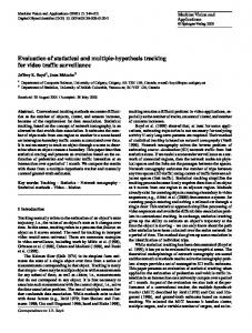
500

9

Velocity RMSE (m/s)

Position RMSE (m)

450

400

350

300 Middle target Right of middle Left of middle

250

200

Figure 2.

Middle target Right of middle Left of middle

8

50

100

7 6 5 4 3

150 200 Time (s)

250

2

300

Position RMSE when separation between targets is 𝑑 = 500 m.

Figure 3.

50

𝑑 = 500 m

150 200 Time (s)

250

300

Velocity RMSE when separation between targets is 𝑑 = 500 m. Table II AVERAGE T RACK L IFE T IME ( S )

Table I T RACK P URITY. Target

100

Track purity (%) 𝑑 = 250 m 𝑑 = 100 m

Target 𝑑 = 500 m

Track life time (s) 𝑑 = 250 m 𝑑 = 100 m

Middle target

98.5

90.4

77.9

Middle target

259.6

259.3

Right of middle

99.2

94.9

82.7

Right of middle

256.8

250.8

255.9

Left of middle

99.3

94.6

85.5

Left of middle

259.8

258.9

256.5

normalized. Any unassigned measurements from the first of the two scans of measurements are used to start new tracks. To initialize the AP-UKF the procedure described in Section III-A2 is used, since no bearing information is available after scan 𝑘 = 1. The purely non-informative prior is used with the initial angle domain taken to be the whole angular space [−𝜋, 𝜋]. A track that is updated with at least three measurements since initialization is considered a confirmed track, while tracks that are not assigned to a measurement in three consecutive scans are deleted. B. Performance metrics calculation The track accuracy and maintenance capability of the proposed algorithm are evaluated by calculating the position and velocity root mean squared errors (RMSE), the average track length, track purity, and track completeness. To calculate the metrics only the confirmed tracks are considered. Number of measurements originated from various targets that are used to update each confirmed track is determined, and the track is assumed to correspond to the target whose measurement contribution to the track is the highest. For each of the three targets once a corresponding track is found, the position and velocity RMSE are found straightforwardly. The track purity is defined as the percentage of measurements used to update the track that originated from the target it is identified to follow. The track completeness refers to the proportion of the targets that are followed by valid tracks at each time step.

253.8

C. Results Figures 2 and 3 show the position and velocity RMSE calculated over 100 Monte Carlo runs when the target separation distance 𝑑 is set to 500 m. One can observe that the target on the right of middle has a much faster convergence of its RMSE than the other two, which is due to the fact that it is closer to the radar platform and hence, has a larger component of the observer acceleration. Table I lists the track purity for the three targets. For the case 𝑑 = 500 m, all three targets have at least 98% purity meaning that data association is performed effectively. Table II lists the average lifetime for each track and it is evident the tracks follow the targets for almost entire duration. Note that the total track length is taken to be the total measurement time of 260 s, and not the total simulation time. Table III shows the number of Monte Carlo runs in which a track that follows each target came to existence. Given that 𝑃𝐷 is 0.9 on average in 90% of the runs each target will have a measurement in the very first scan. It is evident from tables II and III that nearly 90% of the time the tracks initialized in the very first scan have been held throughout. An entry in the column ‘Never’ in this table indicates the number of Monte Carlo runs in which a track has not been held for the target, i.e., indicating track completeness [15]. Out of the 100 Monte Carlo runs a track is not held for one of the targets in only one of the Monte Carlo runs. The separation between the targets has been changed from 500 m to 250 m and then to 100 m. Fig. 4 shows the position RMSE averaged over the three targets for all the three

2131

Table III T RACK I NITIALIZATION T IME

𝑘=1

Number of Monte Carlo Runs 𝑘 = 41 𝑘 = 42 𝑘 = 43

Never

𝑑 = 500 m

Middle target Right of middle Left of middle

92 89 92

7 9 6

1 2 1

0 0 0

0 0 1

𝑑 = 250 m

Middle target Right of middle Left of middle

90 88 92

10 8 6

0 2 1

0 2 0

0 0 1

𝑑 = 100 m

Middle target Right of middle Left of middle

91 83 90

5 16 5

3 1 3

1 0 1

0 0 1

500 d = 500 m d = 250 m d = 100 m

d = 500 m d = 250 m d = 100 m

7

Velocity RMSE (m/s)

Position RMSE (m)

450

400

350

300

6

5

4

50

100

150 200 Time (s)

250

3

300

50

100

150 200 Time (s)

250

300

Figure 4. Average position RMSE of the three targets when the separation distance 𝑑 is varied.

Figure 5. Average velocity RMSE of the three targets when the separation distance 𝑑 is varied.

separations, whereas Fig. 5 shows the average velocity RMSE. It can be observed that as the separation distance is reduced the errors are increased. This is expected since with a shorter separation chances of misassociation increased, which leads to higher errors. The performance is not, however, significantly affected with the maximum position RMSE difference between 𝑑 = 500 m and 𝑑 = 100 m around 100 m. Tables I, II, and III also lists the track purity, average track lifetime, and track initialization times for target separation of 250 m and 100 m. Track purity is degraded when target separation is decreased, with maximum degradation on the middle target. This is because the track following the middle target has greater chance of being misassociated with measurements from either of the adjacent targets. The track life time has also been shortened with the decrease in separation distance. Fig. 6 shows the position and velocity RMSE of the three targets when the separation distance is 500 m for the case of 𝑃𝐷 = 0.8. It is clearly seen that the RMSE of all three targets have increased. Interestingly, now the middle target, although it is closer to the radar platform than the target on the left, has higher position and velocity RMSE. This is because the track following the target in the middle can compete for

measurements from either of the other two targets and has a higher chance of being misassociated. This is evident from the fact that its track purity is only 89%, whereas that for the right and left targets is 95% and 96%, respectively. Also, due to the misassociation to the measurements of one of the other two targets, the track following the middle target is able to prolong its lifetime. The track lifetimes for the three targets are: 216.8 s (middle), 195.6 s (right), and 194.8 s (left). In eleven Monte Carlo runs a track has not been held for one of the targets. V. C ONCLUSIONS We considered the problem of multitarget tracking using range and range-rate measurements, which, unlike the bearings-only tracking, has not received much attention in the literature. A realistic scenario with an unknown number of targets and measurement origin uncertainty was studied. The proposed algorithm considered different cases for track initialization (with or without coarse bearing measurements), uses an AP-UKF for filtering, and the MFA algorithm for finding the association between tracks and measurements. The assignment cost was modified to account for angle-parameterized tracks.

2132

800

11 Middle target Right of middle Left of middle Velocity RMSE (m/s)

Position RMSE (m)

700

Middle target Right of middle Left of middle

10

600

500

9 8 7 6

400 5 300

50

100

150 200 Time (s)

Figure 6.

250

4

300

50

100

150 200 Time (s)

250

300

Position and velocity RMSE of the three targets when 𝑑 = 500 m and 𝑃𝐷 = 0.8.

The performance of the algorithm was evaluated using simulations and the results indicate the effectiveness of the proposed algorithm in terms of tracking accuracy and track maintenance capability. Furthermore, the algorithm was found to be robust against target separation, which illustrates the power of the MFA data association algorithm in the context of this problem. R EFERENCES [1] V. Aidala and S. Hammel, “Utilization of modified polar coordinates for bearings-only tracking,” IEEE Trans. Autom. Control, vol. 28, no. 3, pp. 283–294, Mar. 1983. [2] Y. Bar-Shalom and X. R. Li, Multitarget-Multisensor Tracking: Principles and Techniques. Storrs, CT: YBS Publishing, 1995. [3] D. Bertsekas, “The auction algorithm: A distributed relaxation method for the assignment problem,” Annals of Operations Research: Special Issue on Parallel Optimization, vol. 14, no. 1-4, pp. 105–123, Jun. 1988. [4] S. Blackman and R. Papoli, Design and Analysis of Modern Tracking Systems. Boston, MA: Artech House, 1999. [5] R. Deming, J. Schindler, and L. Perlovsky, “Multi-target/multi-sensor tracking using only range and doppler measurements,” IEEE Trans. Aerosp. Electron. Syst., vol. 45, no. 2, pp. 273–296, Apr. 2009. [6] S. J. Julier and J. K. Uhlmann, “A new extension of the Kalman filter to nonlinear systems,” in Proc. SPIE Conf. on Signal Processing, Sensor Fusion, and Target Recognition, vol. 3068, Orlando, FL, Apr. 1997, pp. 182–193. [7] ——, “Unscented filtering and nonlinear estimation,” Proc. IEEE, vol. 92, no. 3, pp. 401–422, Mar. 2004. [8] T. R. Kronhamn, “Bearings-only target motion analysis based on a multihypothesis Kalman filter and adaptive ownship motion control,” IEE Proc. Radar, Sonar, and Navig., vol. 145, pp. 247–252, Aug. 1998.

[9] T. Kurien, “Issues in the design of practical multitarget tracking algorithms,” in Multitarget-Multisensor Tracking: Advanced Applications, Y. Bar-Shalom, Ed. Norwood, MA: Artech House, 1990. [10] K. R. Pattipati, R. L. Popp, and T. Kirubarajan, “Survey of assignment techniques for multitarget tracking,” in Multisensor-Multitarget Tracking: Applications and Advances, Y. Bar-Shalom and W. D. Blair, Eds. Boston, MA: Artech House, 2000, vol. 3. [11] N. Peach, “Bearings-only tracking using a set of range-parameterised extended Kalman filters,” IEE Proc. Control Theory and Applications, vol. 142, no. 1, pp. 73–80, Jan. 1995. [12] D. Reid, “An algorithm for tracking multiple targets,” IEEE Trans. Aerosp. Electron. Syst., vol. 6, pp. 423–432, Dec. 1979. [13] B. Ristic, S. Arulampalam, and N. Gordon, Beyond the Kalman Filter: Particle Filters for Tracking Applications. Artech House, 2004. [14] B. Ristic, S. Arulampalam, and J. McCarthy, “Target motion analysis using range-only measurements: Algorithms, performance, and application to isar data,” Elsevier Signal Processing, vol. 82, pp. 273–296, 2002. [15] R. L. Rothrock and O. E. Drummond, “Performance metrics for multiple-sensor, multiple-target tracking,” in Proc. SPIE Signal and Data Processing of Small Targets, vol. 4048, Orlando, FL, Apr. 2000, pp. 521–531. [16] T. L. Song, “Observability of target tracking with range-only measurements,” IEEE J. Ocean. Eng., vol. 24, pp. 383–387, Jul. 1999. [17] E. A. Wan and R. Van Der Merwe, “The unscented Kalman filter for nonlinear estimation,” in Proc. IEEE Adaptive Systems for Signal Processing, Communications, and Control Symposium, Lake Louise, AB, Canada, Oct. 2000, pp. 153–158.

2133