Multiple Imputation in the Anthrax Vaccine Research Program

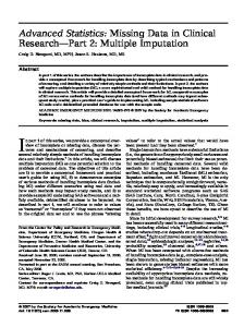
Multiple Imputation in the Anthrax Vaccine Research Program Michela Baccini, Samantha Cook, Constantine E. Frangakis, Fan Li, Fabrizia Mealli, Donald B. Rubin, and Elizabeth R. Zell

Bacillus anthracis under a microscope

A

nthrax, caused by the bacterium Bacillus anthracis, can be a highly lethal acute disease in humans and animals. Prior to the 20th century, it led to thousands of deaths each year. Anthrax infection became extremely rare in the United States in the 20th century, thanks to extensive animal vaccination and anthrax eradication programs. The 2001 anthrax attacks in the United States drew this formidable disease back into the public spotlight. Anthrax spores have not long been used in biological warfare or as a terrorism weapon, but anthrax has been on the bioterrorism (BT) agent list for a long time. U.S. military personnel are now routinely vaccinated against anthrax prior to active service in places where biological attacks are considered a threat. The current FDA-licensed vaccine, anthrax vaccine adsorbed (AVA), is produced from a nonvirulent strain of the anthrax bacterium. The licensed regimen for AVA is subcutaneous administration of a series of six primary doses (zero, two, and four weeks and six, 12, and 18 months), followed by annual booster doses. In 1998, a pilot study conducted by the U.S. Department of Defense provided preliminary data suggesting AVA could be given intramuscularly and without the two-week dose, reducing adverse events and not adversely impacting immunogenicity. Since 2000, the CDC has been planning and conducting a clinical trial, the Anthrax Vaccine Research Program (AVRP), to evaluate a reduced AVA schedule and a change in the route of administration in humans. The AVA trial is a 43-month

16

VOL. 23, NO. 1, 2010

Getty Images/Duncan Smith

prospective, randomized, double-blind, placebo-controlled trial for the comparison of immunogenicity (i.e., immunity) and reactogenicity (i.e., side effect) elicited by AVA given by different routes of administration and dosing regimens. Administration is subcutaneous (SQ) versus intramuscular (IM). Dosing regimens require as many as eight doses versus as few as four doses. In the AVRP, sterile saline is used as the placebo when a dose is not actually administered. The trial is being conducted among 1,005 healthy adult men and women (18–61 years of age) at five U.S. sites. Participants were randomized into one of seven study groups. One group receives AVA as currently licensed (SQ with six doses followed by annual boosters). Another group receives saline IM or SQ at the same time points as the currently licensed regimen. The five other groups receive AVA IM: one group at the same time points as the currently licensed regimen and the remaining groups in modified dosing regimens. Placebo is given when a dose of AVA is omitted from the licensed dosing regimen. There are 25 required visits over 42 months, during which all participants receive an injection of vaccine or placebo (eight injections total), have a blood sample drawn (16 total), and have an in-clinic examination for adverse events (22 total). Total anti-protective antigen IgG antibody (anti-PA IgG levels) is measured using a standardized and validated enzyme-linked immunosorbent assay (ELISA). The primary study endpoints are four-fold rise in antibody titer, geometric mean antibody concentration, and titer. All adverse events,

including vaccine reactogenicity, are actively monitored. Several reactogenicity endpoints are assessed. Potential risk factors for adverse events (e.g., sex, pre-injection anti-PA IgG titer) also are recorded. The AVRP is significant because it is expected to provide the basis for consideration of a change in the route of AVA administration from SQ to IM and of a reduction in the number of vaccine doses. However, as with other complex experimental and observational data, the AVRP data creates various challenges for statistical evaluation. One such challenge is how to handle the missing data generated by dropouts, missed visits, and missing responses. The simplest complete data analysis that drops any subjects with missing data is not applicable here, because even though the overall missing rate is low at this time (3.4%), only 56 among the approximately 2,000 variables are fully observed and only 208 subjects have fully observed variables. Filling in missing values by copying the last recorded value for a subject on a particular variable (the “last observation carried forward” approach) likely is not a good idea in this situation, because side effects and immune response likely will vary over time and not remain constant. Randomly choosing a case with observed data to serve as a donor of values to a case with missing data (the “hot-deck” strategy) could be problematic due to the high degree of missing values and the need to express uncertainty after imputation. During the last two decades, multiple imputation (MI) has become a standard statistical technique for dealing with missing data. It has been further popularized by several software packages (e.g., PROC MI in SAS, IVEware, SOLAS, and MICE). MI generally involves specifying a joint distribution for all variables in a data set. The data model is often supplemented by a prior distribution for the model parameters in the Bayesian setting. Multiple imputations of the missing values are then created as random draws from the posterior predictive distribution of the missing data, given the observed data. MI has been successfully implemented in many large applications. Two such applications are described in “Filling in the Blanks: Some Guesses Are Better Than Others” and “Healthy for Life: Accounting for Transcription Errors Using Multiple Imputation,” both published in CHANCE, Vol. 21, No. 3. MI for the AVRP substantially increases the challenge, mostly due to the large number and different types of variables in the data set, the limited number of units within each treatment arm (Imputations should be done independently across treatment arms to avoid cross-contamination among groups.), and, most important, theoretical incompatibility in the imputation algorithms used by current available packages such as IVEware and MICE. Another important issue is how to evaluate the imputations, a question that has been largely neglected in most of the MI applications.

High-Dimensional Imputation Consider a data set with K variables, labeled Y1, ..., YK , each defined as a vector over a common set of N subjects. Each entry can be missing or observed, so M1, ..., Mk are the vectors such that Mk,i is 1 or 0, indicating whether Yk,i is missing for subject i.

Since 2000, the CDC “ has been planning and conducting a clinical trial, the Anthrax Vaccine Research Program (AVRP), to evaluate a reduced AVA schedule and a change in the route of administration in humans.

”

Imputation with a Joint Model Probability models for two parts of the problem need to be specified to do imputation. First, one can postulate a model (also called a likelihood) for the joint distribution of the variables, given some parameters: pr(Y1, ..., YK | θ), where θ is a vector of model parameters. One also specifies a prior distribution pr(θ) for the model parameters. The prior distribution can express what is known about the parameters. In other cases, a prior distribution is specified in a manner to have little impact on the analysis, but to enable computation of posterior predictive distributions for missing values. For example, if the Yi have independent Bernoulli distributions with an unknown probability of success θ1, then a common choice for the prior distribution of θ1 is a Beta(α, β) distribution. Small values of alpha and beta correspond to a prior distribution with little influence over the analysis. For another example, if all the Y variables have binary outcomes, pr(Y1, ..., YK | θ) could be specified by a loglinear model. The parameters of the log linear model are the components of the vector θ. Second, one needs to consider why the data are missing. Assumptions about why the data are missing are translated into a probability model for the indicator vectors M1, ..., MK. The probability distribution for these vectors is often referred to as the missing data mechanism. An ignorable missing data mechanism is an assumption that the data missing are missing not because of what values would have been observed had they been observed, but because of factors associated with the observed data. This assumption can include the existence of different missing rates for different known groups. If a large collection of covariate variables are available for subjects, such as characteristics collected at study baseline, it is fairly common to assume an ignorable missingness mechanism and build a statistical model to predict response. It is often convenient to generate the imputations using simulation techniques, such as a Gibbs sampling algorithm. CHANCE

17

Figure 1. A missing data pattern that is transformable to a fully monotone missing data pattern. In the transformation, both variables and units are reordered.

In the current application, a Gibbs sampler is defined by the following steps: 1. Start at preliminary values for the missing data of the variables Y– k, where Y– k is defined to be all Ys except for Yk 2. For k =1, ..., K: Generate a random value, θ˜, from the current estimate of the posterior distribution pr(θ | Yk,Y– k,M), which is based on the likelihood, the assumptions about the missingness mechanism, and the prior pr(θ) 3. Simulate the missing values of Yk from the current estimate of the posterior predictive distribution pr(Yk | Y– k,θ˜) When the missing data are ignorably missing, Step 2 can ignore the missingness mechanism and M can be omitted from the notation. As described in Bayesian Data Analysis, the repetition of steps 2 and 3 generally produces simulated values of the missing data that converge in distribution to their posterior predictive distribution under the model.

Practical Complications with High Dimensions When there are many variables to be imputed, finding a plausible model for the joint distribution pr(Y1, ..., YK | θ) is difficult to accomplish for two common ways of postulating joint models. One such way, which postulates a joint model on all variables simultaneously (e.g., a multivariate normal model), is not flexible enough to reflect the structure of complex data such as the AVA data, which include continuous, semicontinuous, ordinal, categorical, and binary variables. A second way is to postulate a joint model sequentially: Postulate a marginal distribution for Y1 first, then a conditional distribution for Y2 given Y1, and so on. If the order of postulation matches the order of a monotone pattern (a special case of missing data pattern), then this way is workable and efficient. This is the fundamental basis for SOLAS. However, 18

VOL. 23, NO. 1, 2010

if the pattern is not monotone, then one has to compute the complete conditional distributions pr(Yk | Y– k,θ), which is often impractical because of the complex relation among the parameters of these models. These complications have led researchers to all but abandon the effort to postulate a joint model. Instead, they follow the intuitive method of specifying directly—for each variable with missing values—the univariate conditional distribution pr(Yk | Y– k,θ) given all other variables. Such univariate distributions take the form of regression models and can accurately reflect different data types. The approaches used with such postulations then follow steps 2 and 3. Software such as IVEware and MICE impute missing data this way. There is a catch, though. If one chooses the conditional distributions pr(Yk | Y– k,θ) for k =1, ..., K directly, there is generally no joint distribution “compatible” with them (i.e., whose conditional distributions pr(Yk | Y– k) equal those of the models chosen). This disagreement is called “incompatibility.” In addition to being theoretically unsatisfactory, incompatibility has the practical implication of the repetition of steps 2 and 3 not generally leading to a convergent distribution. Some methods choose a particular ordering of variables, starting the imputation by the variables with the least missing values to aid convergence. However, the deeper problem of incompatibility is currently ignored. In “Fully Conditional Specifications in Multivariate Imputation,” published in the Journal of Computational and Graphical Statistics, S. Van Buuren and colleagues have presented evidence that in simple cases with ‘good’ starting values, the procedure works acceptably well in practice.

Monotone Missingness Blocks An important case to note is a special type of missing data pattern, depicted in Figure 1. In this pattern, one observes that if, for subject i, the variable Y is missing, then the variable Y is also missing. That is, if k,i k+1,i if M=1, then M =1. Roderick Little and Donald Rubin call such a pattern a “monotone missing data

Figure 2. A simple geometric example to illustrate the concept of continuity, which states that objects defined to be relatively similar to one another should have relatively similar properties.

Figure 3. A missing data pattern transformed to monotone blocks pattern of missing data guided by the concept of continuity.

CHANCE

19

Table 1—Summary of Missing Data and Monotone Blocks by Treatment Arm in Currently Available AVA Data

Treatment Arm 0 1 2 3 4 5 6

Number of Subjects 165 170 168 166 167 85 84

Number of Missing values 927 1372 1558 1383 1325 252 334

Number of Percent in 1st Percent in First 3 Patterns monotone block monotone blocks 15 45 75 13 74 84 13 65 85 15 79 90 15 74 89 7 74 91 9 87 93

Table 1: Summary of missing data and monotone blocks by treatment arm in currently available AVA data.

k,i k+1,i pattern” in Statistical Analysis with Missing Data. The set of rectangles in the right side of Figure 1 is called a “block.” The pattern in Figure 1 is called a monotone block pattern.

Monotonicity and Compatible Sequential Models With a monotone pattern, the likelihood of the data under ignorability can be factored sequentially as the product of the following terms: (i) the product of pr () for subjects with observed y1

The Proposal of Monotone Blocks

(ii) the product of pr () for subjects with observed y1 and y2

The proposal of monotone blocks is a natural extension of Rubin’s method of multiple imputation using a single major monotone pattern (MISM), which exploits a single major monotone block. One can eliminate incompatibility by rearranging the data set to have a completely monotone pattern. On the other hand, deviations from monotonicity can have degrees. Thus, if one rearranges a data set, such as in Figure 3a, to a pattern close to monotone, such as in Figure 3a’, one will be close to eliminating incompatibility. This argument relates to the example of continuity in Figure 2 if one makes the following relations:

(iii) the product of pr () for subjects with observed y1 and y2 and y3 Suppose now one postulates models pr(Yk , ..., Y– k,θ) for k =1, ..., K (i.e., in the order that matches the monotone order of missingness). If one assumes the parameters θk are independent in the prior distribution, each model can be fitted separately from the nine subjects’ data as indicated in (i)–(iii), leading to imputations of missing values, with no need to iterate a Gibbs sampler. Moreover, the sequential postulation of the models ensures full compatibility. This advantage is strictly limited to the monotone missing data pattern. However, it sheds light on how one could design the imputations to minimize incompatibility.

Continuity as a Guide to Approach an Ideal Case For this application, a field of study satisfies continuity if objects defined to be relatively similar have relatively similar properties. An illuminating example of continuity relates to isoperimetric problems, as shown in Figure 2. The first problem asks how to shape a fully flexible fence (Figure 2a) so it encloses maximum area; the answer is a circle (Figure 2a’). Suppose now that, instead of a fully flexible fence, one has a fence that connects eight equal straight segments at flexible joints (Figure 2b), and suppose one asks how to shape this fence13 to enclose maximum area. Observe that the second fence can be 20

thought of as similar to the first, except for the inflexibility along the segments. Now, assuming the Euclidean geometry is continuous for such problems, one should expect that the best shape with the restricted fence would be similar to the best shape with the unrestricted fence. Indeed, the best shape with the restricted fence is the regular octagon (Figure 2b’), which in some sense is the closest shape to the circle, given the constraint.

VOL. 23, NO. 1, 2010

Relate “if one can rearrange the data set to have a completely monotone pattern” to “if one can rearrange the fence to be completely circular” Relate “then one can eliminate incompatibility” to “then one can maximize the area within the fence” Therefore, to apply the argument of continuity here, one first identifies a rearrangement of the data set such that the missing values not forming part of a monotone block are minimal. The part that is monotone is labeled the “first” monotone block. In Figure 3a, the first monotone block consists of the top pattern of missing values, and the bottom pattern of missing values are those that do not form part of the first monotone block. For those missing values, one repeats the process, identifying a rearrangement so most form a monotone block, with the rest of the missing values being minimal. The process

continues until all missing values have been identified with a monotone block. In the AVA data, we applied this process separately for each treatment arm. The information about the missing data and the monotone blocks of the currently available data is shown in Table 1. As one can see, even though the total number of monotone blocks can be large, the first monotone block usually dominates, covering a large proportion of all missing data. On average, the first three monotone blocks include more than 85% of the missing values in each arm. After the monotone blocks were obtained, we imputed the missing data within each block for each arm as follows: (i) Start with filling the missing data of all but the first monotone block with preliminary values (ii) Fit Bayesian sequential models and simulate the missing values for the first monotone block using steps corresponding to steps 1–3 (iii) Treat the data imputed for the first monotone block as observed and impute the missing values for the second monotone block (iv) Continue across all the monotone blocks We then iterated steps (ii), (iii), and (iv) until we detected that the simulations had converged to the desired distributions.

Flexible Regression Models A benefit of modeling univariate conditional distributions instead of large joint distributions is that it is easy to specify and fit different types of outcomes with different types of models. We classified the outcome variables in the AVA data into the following types, according to the models we planned to apply: 1. Binary outcome with two observed levels 2. Categorical outcome with either three (ordered or unordered) levels, or four unordered levels 3. Ordered categorical outcome with at least four, but at most 11, observed levels that have a natural ordering 4. Continuous outcome, defined here as an ordered outcome with more that 11 observed levels and with no extreme level having an observed frequency of at least 20% 5. Mixed continuous outcome—an ordered outcome with more that 11 observed levels and with one of the two extreme levels having an observed frequency of at least 20% Different models are used for different types of outcome variables. For unit i, an outcome variable is denoted by Yi and the set of predictors by the vector Xi. Of course, in this conditional modeling approach, an outcome variable in one model can be used as a predictor variable for a different outcome. In

that case, the variable can be denoted Yi for one situation and included in the Xi vector in the other. A binary outcome is assumed to follow a logistic regression likelihood given covariates Xi, with a “pseudocount” prior distribution for the regression coefficients. The logistic regression likelihood specifies that the probability that Yi is equal to 1 given the values of Xi is logit{pr(Yi =1 | Xi,β)} = X’i β

(1),

where β is a vector of logistic regression coefficients and the logit function of a probability p is ln(p/(1 – p)). This is the standard transformation used in logistic regression. The inverse of this transformation is pr(Yi = 1|Xi,β) = exp(X’i β)/ 1 + exp(X’i β)). The likelihood is the product over all patients of pr(Yi =1|Xi,_) when Yi is 1 and 1 – pr(Yi =1|Xi,β) when Yi is 0. The pseudocount prior distribution essentially imagines the existence of additional prior observations, some with Yi equal to 1 and some equal to 0. The appendix to the 2004 edition of Rubin’s book Multiple Imputation for Nonresponse in Surveys describes this prior specification further. Based on the implied posterior distribution for β, a random value of β is drawn using an iterative simulation algorithm. Based on the draw of β, the missing values of Y are imputed independently across subjects from the logistic regression model. That is, for each subject, given a value of β, the probability that Y is 1 is computed. Using this probability, a Bernoulli random variable is generated as 1 or 0. A categorical outcome with three levels or four or more (L) unordered levels is completely characterized by L – 1 sequential binary regressions. Specifically, one can completely characterize such an outcome by a variable describing “whether the person belongs in level 1.” Then, a variable describing “whether the person belongs in level 2 among those who do not belong in level 1” and so on until all levels have been described. Each regression is fitted as described for the binary logistic regression type. A missing value for Yi is then imputed by simulating sequentially the indicators for the events {Yi =1}, ..., {Yi = L – 1} until one indicator is drawn as 1. If all the indicators are drawn as 0, then Yi is set to L. A categorical outcome with four or more ordered levels is modeled as the continuous type variable. This modeling is preferred to a proportional odds or probit fit for computational stability. The imputed values will be rounded to the nearest level observed in the data. A continuous outcome is assumed to follow a normal regression likelihood given covariates Xi , with a pseudocount prior distribution for the regression coefficient β and the logarithm of the residual variance σ2. Based on a random draw of β and σ2, the missing values of Y are imputed independently across subjects from the normal model. For a mixed continuous-binary outcome, one assumes here that the extreme value with at least 20% of the mixed outcome variable Y is 0 and the remaining values are positive. The model assumed for this type is a logistic regression for Y being at 0 and a normal regression for the log of the positive values of Y. The posterior distribution for the parameters is obtained by fitting these models separately, the first model to the indicator of Y being positive and the second model to the subjects with positive values of Y. A missing value of Y is then imputed by CHANCE

21

is defined “ asFittability invertibility of the corresponding design matrix. It is checked sequentially on the subsets of predictors sorted by AIC in a backward fashion.

”

first imputing the indicator of the value being 0 or positive, and, if positive, imputing a value using the normal regression. Fitting and imputation using each model is as described for the binary and continuous case above. As there are around 2,000 variables and only 1,005 subjects in the AVA data, we constrained the number of predictors that entered the conditional model for each outcome. The predictor selection took place before the imputation procedure. It was based on a preliminarily imputation of all the missing values from their empirical marginal distributions. We allowed the predictors for each outcome variable to differ across different arms and monotone patterns. Demographic variables (i.e., age and sex) were fully observed and always included in the model. For each outcome with missing values, the potential predictors were all the variables that were more observed (i.e., with less missing values) than the outcome. Ideally, we would have selected from the potential predictors by a stochastic search method such as the stepwise regression based on the Akaike’s information criterion (AIC). The computational demand of conducting such a search among 2,000 variables for each outcome in each monotone block, however, was prohibitively large. Instead, we fit the regression models of the outcome given each single potential predictor—age and sex—and sorted the predictors according to the corresponding AIC’s. Then, the 20 predictors with the smallest AIC were selected. Finally, we checked the “fittability” of the conditional model, which contemporarily includes all the selected predictors on the complete cases. Fittability is defined as invertibility of the corresponding design matrix. It is checked sequentially on the subsets of predictors sorted by AIC in a backward fashion. If one predictor is not “fittable,” it does not contain enough information on the outcome and is selected mostly because of the model assumption. Therefore, this predictor is dropped from the subset and the same checking goes on to the next selected predictor until the last one. This checking procedure is done separately within each treatment arm and monotone pattern. 22

VOL. 23, NO. 1, 2010

Software coded jointly in R and Fortran has been developed to address each of the univariate problems (i.e., one imputation of one outcome in one treatment arm). Several simulation studies show the software handles data well.

Evaluation Plan Evaluating methods is always as important as developing them. Much work has been done in proposing and applying imputation methods, but remarkably little in corresponding evaluations. Comparing the imputed values to the observed values (i.e., the ‘truth’) is the most intuitive evaluation, but is neither generally possible nor a valid method of evaluation. Instead, one simulates missing data in a fully observed subset of the data set and imputes these created missing data. Then, one compares the inferences based on the imputed data set to the inferences based on the original, complete data set. A similar approach was taken in the Third National Health and Nutrition Examination Survey (NHANES III) evaluation by Andrew Gelman and Rubin in the Statistical Methods in Medical Research journal article “Markov Chain Monte Carlo Methods in Biostatistics” and by Trivellore Raghunathan and Rubin in their article, “Roles for Bayesian Techniques in Survey Sampling,” which appeared in the proceedings of the Silver Jubilee Meeting of the Statistical Society of Canada. To avoid conflict of interest, the AVA team was split into two subteams: the evaluation team and the imputation team. The evaluation team first created artificial missingness in a subset of complete data. The imputation team, blinded to the truth, then imputed the created missing data. After that, the evaluation team took over again. They derived and compared the inferences based on the imputed and complete data. The evaluation team first defined a set of key variables (Y1, ..., Yt), the values of which are of primary interest in the analysis. Then, they identified the missing patterns of the key variables presented in the data set. A missing data pattern is a unique vector of the t corresponding missing indicators. There are at most 2t missing patterns of t variables. For example, in the analysis of the immunogenicity of AVA, the CDC defined the Elisa measurement at four weeks, eight weeks, six months, and seven months as the key variables. A unit (person) who has Elisa measurement for, say, the first three time points belongs to the missing pattern (0, 0, 0, 1). Defining the complete subset as the set of units whose key variables are fully observed, the evaluation team then simulated 200 copies of the complete subset with varying missing data patterns and proportion of missingness as follows: Step 1: Count the numbers of units that belong to each pattern. Rank the missing patterns by their sizes in decreasing order. (Pattern 1 is the most prominent missing pattern.) Step 2: For pattern j =0, ..., J (0 means fully observed), use logistic regression using a pseudocount prior distribution to model the probability of being in pattern j versus being in patterns j +1, ..., J given all covariates X. Denote the estimated intercept and coefficients (αˆ j,βˆ j). The estimated probability of a unit i being in pattern pi,j is logit–1((αˆ j,βˆ j) (1,Xi)T ).

Step 3: Choose α0 that gives the overall proportion of missing data approximately equal to 10%. For each unit i, calculate its probability of being fully observed: logit–1((α0,βˆ 0) (1,Xi)T ). Then, randomly assign the missing indicator =0 to the units based on these probabilities. Next, for each unit that is assigned to be missing (i.e., not fully observed), calculate its probability of belonging to missing pattern 1—logit–1((αˆ 1,βˆ 1)(1,Xi)T )—and randomly assign it to pattern 1 (versus patterns 2 to J). Continue this procedure through pattern J –1. At last, each unit in the complete set belongs to a missing pattern (including the pattern of fully observed) and the overall missing proportion is 10%. Step 4: Choose values of α0 that give overall missing proportions of approximately 20%, 30%, 40%, and 50% and repeat Step 3 40 times for each α0. The imputation team, upon receiving the altered data sets from the evaluation team, used the monotone block imputation procedure to provide five imputed data sets for each of the 200 copies at each value of _0. Finally, the evaluation team calculated the empirical 95% (and 90%, 80%, and 50%) confidence intervals for a set of summarizing functions of each key variable (e.g., a mean) from the imputed data sets. They compared these to the corresponding intervals based on the original, complete data set. Evaluations like this are rarely done, but often give rather disappointing results for standard (nonmissing data) procedures.

Remarks Motivated by the missing data problem arising from the AVA trial, we developed a general approach to handling nonmonotone missing data from data sets that have a large number of variables and many types of data structures. The design of the imputations we used here breaks the nonmonotone pattern into blocks of separate patterns, each of which is monotone and can be handled with sequential modeling. There can, of course, be other ways of building around the ideal case of monotonicity, to address nonmonotone patterns. An interesting problem is to explore generalizable ways of comparing such approaches in how they best reduce the impact of incompatibility. Within monotone patterns, the large number of variables is still an issue. It was handled here in an approach that looks at each regression isolated from the others. Perhaps it would be beneficial from a predictive standpoint to have a more integrated assessment of reducing the dimension of the models. Moreover, one has to ask how answers to these problems can help design the study better. For example, for which variables do the missing data impact most the overall efficiency or compatibility? An easy and generalizable way to answer such questions could suggest, for example, offering increased incentives for the collection of these data or developing proxy measurements that would have higher observation rates. So far, we have focused on addressing the missing values for the variables intended to be measured in the study with human subjects. A practically more important task is to address missing measurements not intended to be obtained in this study— these values are the survival status of the human subjects if, after the vaccination, they had been exposed to anthrax. For predicting this survival, there is little information from the

human study alone because exposing humans to lethal anthrax doses is not ethical, given the risks of such exposure. For this reason, in parallel to the study with humans, CDC has been conducting a study with macaques. The macaque study is similar to the human study with the important exception that after vaccination, the macaques are exposed to anthrax and their response—including survival status—is measured. An important question, therefore, is how to bridge the human and macaque information to estimate the survival of humans if the vaccination regime under study had been followed by an exposure to anthrax. An answer to this question is not trivial and depends on what parts of the model among dosage, immunogenicity response, and survival are generalizable between the macaque and human studies. Thus, advancing knowledge in this problem will have to rely not on a single study, but on how this study is combined with existing knowledge. Editor’s Note: The findings and conclusions in this article are those of the authors and do not necessarily represent the views of their institutions.

Further Reading Frangakis, C. E., and D. B. Rubin. 2002. Principal stratification in causal inference. Biometrics 58, 21-29. Gelman, A. E., J. B. Carlin, H. S. Stern, and D. B. Rubin. 2004. Bayesian data analysis. Boca Raton: Chapman and Hall. Gelman, A. E., and D. B. Rubin. 1996. Markov chain Monte Carlo methods in biostatistics. Statistical Methods in Medical Research 5(4):339-355. Little, R. J. A., and D. B. Rubin. 2002. Statistical analysis with missing data. New Jersey: Wiley. Raghunathan, T. E., and D. B. Rubin. 1998. Roles for Bayesian techniques in survey sampling. Proceedings of the Silver Jubilee Meeting of the Statistical Society of Canada 51–55. Rao, J. N. K., W. Jocelyn, and N. A. Hidiroglou. 2003. Confidence coverage properties for regression estimators in uniphase and two-phase sampling. Journal of Official Statistics 19:17– 30. Rubin, D. B. 1987, 2004. Multiple imputation for nonresponse in surveys. New York: Wiley. Rubin, D. B. 2003. Nested multiple imputation of NMES via partially incompatible MCMC. Statistica Neerlandica 57(1):3–18. Van Buuren, S., J. P. L. Brand, C. G. M. Groothuis-Oudshoorn, and D. B. Rubin. 2006. Fully conditional specifications in multivariate imputation. Journal of Computational and Graphical Statistics 76(12):1049–1064.

CHANCE

23