Proceedings of the 13-th Australasian Data Mining Conference (AusDM 2015), Sydney, Australia
Multiple Imputation on Partitioned Datasets Michael Furner1 1
Center for Research in Complex Systems School of Computing and Mathematics, Charles Sturt University, Bathurst, NSW 2795, Australia, Email:
[email protected]
2
Center for Research in Complex Systems School of Computing and Mathematics, Charles Sturt University, Bathurst, NSW 2795, Australia, Email:
[email protected]
Abstract This paper discusses the impact of making modifications to partition-discovering missing value imputation techniques, and through this process develops a novel imputation algorithm which makes use of partition discovering and multiple imputation - two state of the art techniques. We discuss the difference between global and partition-discovering imputation techniques and show how the techniques have been developed over time through making modifications to existing techniques in the literature. Beginning by examining the role of missing value imputation as it relates to the world’s increasing desire for data analysis, we proceed to review the current state of the art in regards to global and partitiondiscovering imputation techniques, and categorise a variety of existing algorithms into these classes. Provided in this section is an in-depth discussion of an algorithm from each of these categories (EMI and SiMI) in order to gain a greater understanding of how each one works before developing novel techniques. This is followed by the presentation of several variants to the SiMI algorithm, which are used as a launchpad to our discussion of our proposed technique, the MultiSiMI algorithm, which is shown to improve SiMI’s quality of imputation on 6 of 7 datasets tested. This technique is the major contribution of this paper. Each section with a variant of SiMI presents experimental results for the variant discussed in order to gain an understanding of how intelligent modifications to existing algorithms can result in superior novel techniques such as MultiSiMI. We conclude by reviewing the contributions of the paper and recommending some future research directions. Keywords: missing value imputation, data mining, missing values, decision trees, data cleansing, data munging 1
Md Zahidul Islam2
Introduction
As the world becomes increasingly dominated by digital media and technology, so too have we advanced our methods of analysing data for various purposes. c Copyright 2015, Australian Computer Society, Inc. This paper appeared at the Thirteenth Australasian Data Mining Conference, Sydney, Australia. Conferences in Research and Practice in Information Technology, Vol. 168. Md Zahidul Islam, Ling Chen, Kok-Leong Ong, Yanchang Zhao, Richi Nayak, Paul Kennedy, Ed. Reproduction for academic, not-for profit purposes permitted provided this text is included.
In the 21st century technology is so ubiquitous that we are collecting more data than ever before. Data mining algorithms such as decision trees and artificial neural networks give researchers, marketers, and analysts the ability to peer deeply into the patterns that exist in huge datasets, allowing them to find unprecedented levels of new information within the collected records. It may often be thought, however, that data collection is perfect. Being surrounded by the numerous devices we use everyday builds a false sense of security about their reliability. It is in fact the case that whether by fault of the collection hardware, or some information being deliberately omitted by the data subject - datasets are commonly incomplete (i.e. some attribute values are missing). In situations where this is the case it is important that the missing values are preprocessed (for example cleansed ) in order to ensure that the analysis undertaken on the data is more accurate and provides more meaningful results than the analysis on the unprocessed data. If there is noise in the dataset, the noisy values need to be identified as such so that we can either correct for the noise or mark them as if they were missing. When the values are missing or marked as such, the values need to be dealt with - often with a missing value imputation strategy. Historically, a common approach to handling when a record in a dataset has missing values for one or more of its attributes has been to completely remove the record. This trivial solution is known as Complete Case Analysis (Schafer & Graham 2002), and while it seems like an intuitive idea it has several problems. Simply removing records may cause biases towards particular values in attributes, causing a skewed analysis (Schafer & Graham 2002). Substituting attribute means for missing values is another simple approach for dealing with this problem, but it has been shown in the literature to create biased estimates (Tresp et al. 1995). Also, if one attribute is missing in a record and we delete the whole record, we lose the data in the rest of the record. This data may be important or have ramifications for the analysis of the dataset, and in a world where data is money it is hardly an economical approach. Also, it has been shown in the literature that the accuracy of prediction using decision trees improves when imputing the missing values in a dataset rather than leaving them un-imputed (Wang et al. 2014). Because of the limitations of such simplistic approaches to handling missing data, many algorithms have been produced to make a well reasoned estimate
59
CRPIT Volume 168 - Data Mining and Analytics 2015
for the missing values in a dataset. Amongst these methods is the Expectation Maximisation Imputation (EMI) algorithm (Schneider 2001), which performs an iterative imputation on the numerical missing values within a record by using the mean values of the numerical attributes and the correlation matrix of the dataset. By using a cycle of parameter estimation and imputation until convergence, the algorithm makes use of the common and well documented EM technique (Dempster et al. 1977) for the purposes of imputation. Due to EMI’s reliance on the correlation matrix between attributes, several techniques have been developed in order to find horizontal segments of the dataset in which intra-attribute correlation and similarity among the attributes are high. An early one of these was DMI (Rahman & Islam 2011), which used the leaves of a decision tree in order to find these horizontal segments. A more advanced interpretation of a similar concept can be found in SiMI (Rahman & Islam 2013a), which instead finds the intersections between leaves from the different trees of a decision forest and uses these as the segments. SiMI proposes that the records belonging to these intersections are expected to be more similar than those of a single leaf found by DMI, and therefore will provide better results for the EMI imputation (Rahman & Islam 2013a). Another regression-based technique for missing value imputation is IBLLS (Iterative Bi-clustering Local Least Squares) (Cheng et al. 2012). Originally designed for use with microarray gene expression data, this algorithm iteratively finds the nearest neighbours of a record and imputes the missing values within the record using a least squares equation, only taking into account of those attributes within the record that are correlated highly enough with the target attribute (i.e. the attribute with a missing value that must be imputed). This, as well as EMI, can only be used to impute numerical attributes, so another technique must be undertaken to impute categorical ones. As seen in the evolution of SiMI from DMI, and DMI from EMI, intuitive improvements to existing algorithms provide fertile grounds for further research within the field of missing value imputation. This paper aims to build on this tradition by combining the demonstrably powerful approach we identify as partition-discovering with the advanced techniques of multiple imputation. We present three variants of existing techniques, each identifying a key component in previous literature as a basis on which to modify existing algorithms. The first two of these provide examples of how different methods of modification result in a drastically different imputation accuracy result, with a clear improvement from the first to the second based on the nature of the change outlined. Through the process of developing these first two, we lead into our third - in which we show the strength of our proposed technique MultiSiMI, which provides a significant improvement upon the algorithm on which it is based and is the major contribution of the paper. The paper will begin by discussing the different categories of missing value imputation techniques, with an explanation of some techniques that fall within them. The techniques are identified as global and partition-discovering. A large number of modern missing value imputation techniques are placed into these categories to provide a better understanding of the way they work in relation to each other. We then proceed to identify areas for change in existing techniques, and show how our modifications work to achieve a different result.
60
Each section provides experimental results which we use to further understand the impact of the modifications proposed. These results are gathered by running the algorithms in question on datasets we create by inserting missing values in a variety of patterns, ratios and models (Junninen et al. 2004) into publicly available clean datasets (i.e. datasets with no missing values) from the UCI Machine Learning Repository (Bache & Lichman 2013). The patterns used are as follows: a simple pattern, where a record can have at most one missing value; a medium pattern, where if there are missing values in a record then a minimum two and a maximum of 50% of the attributes will be missing; a complex pattern which has a minimum of 50% and maximum 80% attributes in a record with missing values and a blended pattern which has missing records with a mixture of records from the other three patterns, with 25% of the records with missing values being simple, 50% being medium, and 25% being complex (Rahman & Islam 2013a). We also use 4 ratios of missing values (1%, 3%, 5% and 10%) which determine the percentage of total attribute values in the data set that are missing (Rahman & Islam 2013a). In each section, we compare the section’s modifications to SiMI, the algorithm that has been modified in each case. It is important to note that there are multiple mechanisms through which missing values can occur. Missing at random (MAR) refers to when the missing attribute value depends on the other attributes of the record that are missing (Schafer & Graham 2002). Missing Completely at Random (MCAR) makes no such assumptions, meaning we assume that the probability of the value being missing is in no way related to anything else in the data set (Schafer & Graham 2002). Missing Not at Random (MNAR) implies that missing values depend on other missing values so it is subsequently impossible to estimate from those values we have access to (Aydilek & Arslan 2013) (Schafer & Graham 2002). The advanced techniques to be discussed in this paper make the assumption that the mechanism for missing values in the dataset is MCAR - an important factor to note, as a different approach would need to be undertaken for other patterns. The models of missingness used are Overall and Uniformly Distributed (UD). In the UD model, missing values are spread equally over all of the attributes, wherein Overall they are not. With the four missing patterns, four missing ratios and two missing models we have 32 combinations of missingness. Each of these combinations is used to generate 10 missing value data sets with any given clean data set in order to compensate for the randomness in generating the missing value data sets. The 320 missing value datasets created for each original dataset have missing values in an MCAR pattern due to this process, so the application of our missing value imputation algorithms is suitable. We use this methodology for testing as it has been used previously in literature of a similar nature (Rahman & Islam 2011, 2013a, 2014) due to the characteristics of missing data in a dataset having an impact on the performance of the missing value imputation techniques (Junninen et al. 2004). We use the index of agreement (d2 )(Junninen et al. 2004) evaluation criteria to evaluate the use of the algorithms. Other evaluation criteria such as RMSE, MAE and R2 (Willmott 1982) have been used in the literature, but due to space restraints we will use the aforementioned d2 criteria. For this evaluation criteria, we display the average over all 32 combinations, each of which has been averaged over 10 missing value datasets. All of the data sets used are freely available
Symbol D |D| A Aj ri rij f k τ µ Σ w δ R C Ci Cij cˆi
Proceedings of the 13-th Australasian Data Mining Conference (AusDM 2015), Sydney, Australia Meaning by highly similar records in the dataset, as the mean Dataset vector will be very close to the available attribute No. Records in Dataset values. Secondly, the higher the correlation between Set of Attributes attributes, the more accurate the result based on the jth attribute in A regression coefficient matrix B. It is from these obRecord i in D servations that justification for a new collection of Value of attribute j in ri algorithms was developed. Fitness function Number of initial centroids in k-means SiMI (Rahman & Islam 2013a) and its predecesMin. no. records in an intersection/cluster sors take a completely different approach by improvMean vector ing imputation accuracy from previous techniques Covariance matrix not by directly altering a basic algorithm or proposWeight scalar ing a trivial imputation solution, but by providing an Correlation threshold existing algorithm with an environment in which it Correlation Matrix can perform its imputation better. These algorithms Set of Clusters justify this approach by claiming that certain segith cluster in C ments of a dataset typically have higher correlation ID of the jth record of the ith cluster in C Cluster centre of Ci between attributes than their correlation within the
Table 2: Symbol Table from the UCI machine learning repository. See Table 1 for a summary of the data sets used in the experiments. A list of commonly used symbols (Table 2) has been provided to aid in the understanding of the many algorithms discussed in the paper. 2
Background Research: What are PartitionDiscovering Imputation Techniques?
One of the most effective algorithms for missing value imputation is EMI (Nelwamondo et al. 2007). EMI works using the expectation-maximisation algorithm, which iteratively updates parameters based on previous iteration’s results. This algorithm is designed to work on a whole dataset, and provides a novel, global technique to imputation. It accomplishes this by computing the deviation of the available attributes in a record with missing values from their means, weighted by the correlation between the available attributes and the missing attributes. This correlation is derived from the covariance matrix Σ, and we split the mean vector µ into those attributes that are available in the record (µa ) and those whose values are missing in the record (µm ). We index the covariance matrix Σ as follows: Σaa is the covariance matrix between available attributes in the record, Σam is the covariance matrix between those attributes available and those missing, Σmm is the covariance matrix between missing attributes in the record, and Σma is the covariance matrix between missing attributes in the record and available attributes in the record. A vector of missing attributes in a target record ri , xm is estimated using the following equation: xm = µm + (xa − µa )B + e
(1)
Where xa is the available attributes in the target record, B is defined as Σ−1 aa Σam and e is a random residual vector with 0 mean and covariance matrix Σmm − Σma Σ−1 aa Σam considered only on the first iteration (Schneider 2001). After each iteration of the algorithm, EMI recalculates the mean vector µ and the covariance matrix Σ, allowing the next iteration to use a more accurate estimate for the true mean vector and covariance matrix in its imputation. This process continues until there is no longer any change between iterations, meaning we have found the imputation with maximum likelihood based on the process. A quick inspection of the equation indicates two things. First, the term (xa − µa ) will be minimised
whole dataset. They also argue that this property improves the efficacy of EMI as EMI uses the correlation between attributes as a primary component of its imputation calculation (Rahman & Islam 2011), as we previously observed. An example of this property would be the correlation between age and height. Within a dataset representing people, records with an age below 20 will likely have a high correlation between age and height that does not exist in the rest of the dataset. Similarly, SiMI proposes that these groups will also have highly similar records, providing even further justification. SiMI’s process works as follows. First, the dataset is divided into two parts; in one part we have all the clean records that have no missing values, and in the other we have all records that do have missing values. Then, SiMI builds a decision forest (Islam & Giggins 2011) on the clean records in the dataset, and once we have the rules for the decision trees in the forest, we assign the missing value records to their appropriate leaves. Each tree in the forest will have leaf whose logic rule satisfies the attribute values of a record ri . We say that this record ri belongs to the leaf, so therefore each leaf represents a set of records whose attribute values are satisfied by the leaf’s logic rule. The record ri belongs to one and only one leaf of each tree, but since there are n trees in a decision forest, ri belongs to n leaves, one from each tree. SiMI will then take the intersection of each of these n sets of records. Now, ri belongs to one and only one intersection, and this intersection is considered by SiMI to consist of highly similar records to ri . As some of these intersections may be very small, SiMI uses a merging algorithm to merge intersections that have less than a user defined value τ records. In considering which intersection that the smallest intersection with less than τ records should merge with, SiMI implements a user defined weight λ. They consider two criteria for selecting the best intersection to merge with, and use λ to determine the strength of these criteria on the selection process. The first of these criteria is similarity between intersections (Sim), in which we calculate the normalised recordto-record distance from one intersection to the other (dj ) and find the similarity via (1 − dj ). The second criteria is correlation (Cor), which is determined by the L2 norm of the correlation matrix for the new intersection that would be created if the two candidate intersections were merged. These criteria are combined as follows: V = Sim × λ + Cor × (1 − λ)
(2)
SiMI merges the smallest intersection with the intersection that provides the highest V value. This
61
CRPIT Volume 168 - Data Mining and Analytics 2015 Dataset Name No. of Records (|D|) Yeast 1484 Pima 768 Credit Approval 653 (CA) Contraceptive 1473 Method Choice (CMC) Heart 270 German CA (nu- 1000 meric) Auto MPG 392
No. Numerical Attr. 8 8 6
No. Categorical Attr. 1 1 10
Total Attr. 9 9 16
2
8
10
6 24
8 1
14 25
5
3
8
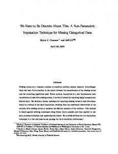
Table 1: Summary of data sets used process iterates until there are no more intersections with less than τ records. Once this merging is completed, SiMI performs an imputation with EMI to deal with missing numerical values, and a mode imputation (from just within the intersection) in order to deal with categorical attributes. Figure 1 shows how SiMI finds intersections with which to perform these operations on. Missing value imputation algorithms can be grouped into two sometimes overlapping categories. The first category is global techniques, which use the entire dataset provided in order to impute the missing values. Algorithms such as EMI, least-squared imputation (Cai et al. 2006) (another regression technique), FIMUS (Rahman & Islam 2014), mean imputation (Schafer & Graham 2002), mode imputation (Schafer & Graham 2002), hot deck imputation (Schafer & Graham 2002), and Support Vector Regression Imputation (Mallinson & Gammerman 2003) fall into this category. Algorithms that divide the dataset in order to find a better environment to perform a global imputation technique within can be described as partition-discovering, and include DMI (Rahman & Islam 2011), IBLLS (Cheng et al. 2012), ILLS, LLS (Cai et al. 2006), k-NNI, SVDImpute (Troyanskaya et al. 2001), and SiMI (Rahman & Islam 2013b). SiMI was shown in its original paper to provide better results than EMI over many datasets (Rahman & Islam 2013a), and as such we compare against SiMI only in our experiments (as the purpose of the experiments is to improve the imputation quality of SiMI). It is important to preface the following study with a note however - parametric partition-discovering techniques can be temperamental. The following section seeks to address this with the following question: ”are decision trees really the best way to find high similarity horizontal segments?” 3
Using Alternative Methods for Finding High Similarity Horizontal Segments
SiMI and its predecessors use a decision tree or decision forest in order to find horizontal segments (i.e. subsets of records) of a dataset where within each subset the records have high similarity and the attributes are highly correlated. This is in order to increase the effectiveness of the EMI algorithm for imputing numerical attributes, and to provide sets of similar records for a better mode imputation on categorical attributes (Rahman & Islam 2013b). A major issue with the use of decision trees for finding horizontal segments with high similarity is that they are a complex solution to a relatively simple task. The popular decision tree algorithm C4.5 has been extensively studied, and is known to have a complexity of O(|D||A|2 ) (Su & Zhang 2006) where
62
|D| is the number of records in the dataset and |A| is the number of attributes. For a high dimensional dataset the complexity of building a tree can be very high. Moreover, not all datasets have well defined class attributes, so this can also be problematic as if the decision trees have a low prediction accuracy they may not be finding highly similar records within their leaves. SiMI also requires the specification of several parameters, including the parameters for decision tree and decision forest algorithms. This amounts to at least 8 parameters when we take into account SiMI’s own λ and τ values (Rahman & Islam 2013b). Having these parameters set to non-optimal values (which vary from dataset to dataset) can drastically reduce the quality of the imputation produced. The process that SiMI undertakes in order to find horizontal segments is explained in more detail in the previous section, but this startling fact can be a motivating factor in developing new missing value imputation techniques. Clustering algorithms are designed to find distinct sets of close records within a dataset (Jain 2010), and due to this may yield the potential for a better imputation result when combined with a regression algorithm such as EMI as has been done in DMI and its successors, or the least squares regression used in IBLLS. We propose that in the context of missing value imputation, the need to find distinct clusters is less important (i.e. those with high intra-cluster similarity and low inter-cluster similarity) than the need to find groups of highly similar records (i.e. considering high intra-cluster similarity and ignoring intercluster similarity), meaning we can also use a different method for determining the fitness of the set of clusters found. We present a modification to SiMI for the purposes of testing the hypothesis that a clustering algorithm can be used in order to find high similarity horizontal segments, which will be further referred to as kMeans SiMI. For a clustering algorithm, we will use k-means, as it is widely used and has a low complexity of O(|D|) (Jain 2010). The k-means algorithm uses a simple iterative process to find cluster, and as the name suggests takes a parameter for the number of expected clusters, k. The algorithm begins by selecting k centroids from random points from within the dataset, and assigns each records to one of these centroids. The centroids are then recalculated by taking the mean of the attributes of each of the records in their cluster, and this process of assignment and recalculation is repeated until there is no change in the cluster boundaries. These operations are all performed on a normalised version of the dataset. Due to the normalisation process it is possible to naively include categorical attributes in the k-means process by considering a distance of 1.0 to non-matching values and 0 to matching values. However, in this experimentation we do not include categorical attributes in
Proceedings of the 13-th Australasian Data Mining Conference (AusDM 2015), Sydney, Australia
Figure 1: SiMI finding intersections on a basic dataset (Rahman & Islam 2013a). the k-means process since it would place an imbalance onto categorical attributes in the distance calculations. In order to set the k value and to deal with the nondeterministic nature of k-means, we run the algorithm multiple times (10 in ourpexperiments) with various k values (between 2 and |D|) to get several sets of clusters, and select the set of clusters that provides the best score with a fitness function f . This fitness function can be designed in many ways, and will have an impact on both the complexity and effectiveness of the algorithm. One way of determining f is to take into account the intra-cluster similarity between records and their cluster centre, weighted by the ratio of amount of records inside the cluster. Given this, we have:
mode imputation. All tests performed on SiMI in the experiments of this study we use a minimum of 7 decision trees, and a minimum of 100 records in each leaf. In cases where the training dataset (i.e. the clean records of the dataset) is too small to accommodate these parameters, we use a minimum record number between 20 and 5. Forests are generated using the SysFor (Islam & Giggins 2011) algorithm, and trees are generated using C4.5 (Quinlan 1993). The results are shown in Figure 2, with k-Means SiMI (shortened to kSiMI) indicating its fitness function as either f1 (kSiMi f1) or f2 (kSimi f2) from Equations 3 and 4. As mentioned previously, the results in this paper are presented using index of agreement (d), defined for a record ri in (Junninen et al. 2004) as: P|A|
" P|C| P|Ci | f1 =
i
j
sim(rCi,j , cˆi )
|D|
(3)
Another potential fitness function we could use is based on Pearson correlation. This potential fitness function works by taking the average of the norms of the correlation matrix of the clusters. P|C| f2 =
j=1
kRj k2
|C|
(4)
Where Rj is the correlation matrix of the jth cluster. After running k-means multiple times, we select the set of clusters with the highest f value and use this to proceed to the next step. Any cluster in this set that has less than τ records must be merged with another cluster, and we use SiMI’s intersection merging procedure for this. As with SiMI, these horizontal segments have their numerical values imputed using EMI, and their categorical attributes imputed via
d = 1 − P|A|
j=1 (rij
j=1 (|rij
0 z − rij )
0 − µ |)z − µj | + |rij j
# (5)
where z is either 1 or 2,rij is the original value 0 for Aj (before missing values are added), and rij is the imputed value for Aj . We use z = 2, thus the designation d2 . We present the average d2 over the whole dataset, where a higher value is better. Our results show three important characteristics. Firstly, the new variant only provides a consistently better result on the AutoMPG dataset. This may be due to AutoMPG having a small number of records, or due to the dataset having clearly defined clusters. Secondly, on the German CA dataset, the fitness function f1 when used with k-Means SiMI outperforms SiMI, whereas f2 does not. This is in contrast to on the AutoMPG dataset, where in the situation that both fitness functions with k-Means SiMI, f2 outperformed f1 Finally, and as a consequence of the previous two characteristics, we can see that the fitness function appears to have a large impact on the performance of the k-means SiMI algorithm.
63
CRPIT Volume 168 - Data Mining and Analytics 2015
Figure 2: k-means SiMI d2 results (higher the better)
Figure 3: Results of correlation tests within partitions
The results obtained from testing this modification compared with the existing algorithm SiMI are thoroughly interesting, and from them we can derive several meaningful and justified directions for further research. We see that k-means partitioning performs with less efficacy than SysFor partitioning, likely due to the enhanced ability of a decision forest for taking into account categorical attributes for partitioning. Further tests should be completed using categorical attributes during clustering, although we advise the reader to use distance measures which are better suited to categorical attributes rather than the naive approach described earlier for this. Some of these include Eskin (Xiang & Islam 2014), IOF (Xiang & Islam 2014), and Gambryan (Xiang & Islam 2014), each of which has been shown to work with differing degrees of efficacy depending on the nature of the dataset (Xiang & Islam 2014). Perhaps a new, more powerful fitness function needs to be used, taking into account a combination of both similarity and correlation. At any rate, this seems to indicate that further research into the field of missing value imputation with regards to finding horizontal partitions needs to be focused on using more sophisticated methods of finding the partitions, rather than just k-means on numerical attributes with the specified fitness functions. In order to gain an understanding of the results,
we decided to test the average correlation within SiMI intersections and the k-means clusters our algorithm generates (using the norm of the correlation matrix for the subsets). The results of this can be seen in Figure 3. Not surprisingly, SiMI had a higher correlation on most datasets, although there are some peculiarities. Firstly, AutoMPG, the dataset on which the new algorithm performs best, does not have a higher average correlation between attributes inside the k-means clusters. Also, on German CA, Pima and Yeast we find that the k-means clusters have a higher average correlation than SiMI intersections. This may point to something else providing the enhancement in imputation accuracy for EMI, rather than the correlation being high as was suggested previously (Rahman & Islam 2013a). Certainly there are upsides to the k-Means SiMI algorithm. Firstly, in that it is less complex than an algorithm such as SiMI. Secondly, it requires only 3 parameters in comparison to the at least 8 required by SiMI. In the past, in order to improve the horizontal segments found by DMI, a pre-imputation step was used. In the next section we discuss the use of this technique to improve the quality of clustering performed by k-Means SiMI to achieve an improved imputation results.
64
Proceedings of the 13-th Australasian Data Mining Conference (AusDM 2015), Sydney, Australia
4
Consecutive layers of imputation
Techniques such as EDI (Rahman & Islam 2013b) have effectively used multiple consecutive layers of imputation in order to provide a better final imputation result. IBLLS similarly uses a self updating threshold to iteratively perform imputations that improve over time (Cheng et al. 2012). Subsequently, one may expect that by applying the same logic to the dataset before running the clustering algorithm k-means may improve the clusters and thus allow for a better imputation result. EDI works by running a pre-imputation step before creating decision trees. In this step, the entire dataset has its numerical attributes imputed by EMI, and this imputed dataset is passed onto C4.5 to create a decision tree (Rahman & Islam 2013b). The theory behind this technique is that the imputed dataset should provide leaves more suitable for use in the DMI algorithm. The leaves found by the decision tree have the imputed numerical values replaced with their original missing values and are imputed using EMI and categorical attributes are imputed using a mode imputation. This technique can also be applied to the k-Means SiMI algorithm described earlier in order to potentially achieve a better clustering result by allowing us to cluster all of the records at once. We call this new algorithm EKSiMI. We impute numerical attributes using EMI before using k-means to cluster the records, and then merge clusters that are below user defined minimum size τ . We then replace the records that originally had missing values within the final clusters. Finally, we impute as before, using EMI for numerical attributes within clusters and mode imputation using the modes of records within clusters for the categorical attributes. For the k-Means SiMI cluster fitness function, we have used f1 described earlier. The results found on EKSiMI (using the distance based fitness function) provide an interesting result (Figure 4). On most of the datasets, using EMI before the clustering process as a pre-imputation step provides a better final imputation results than standard k-Means SiMI, and makes it significantly more competitive with SiMI. This is likely due to the preimputation step allowing all records to be clustered at once, rather than clustering the clean records and assigning missing value records to the closest cluster afterwards. We see the results of EKSiMI as promising, and indicative of the potential of using cluster-based partition-discovering techniques in the future. Future cluster-based partition-discovering techniques should however attempt to use a pre-imputation step for potentially better results. Perhaps with this preimputation step and a better fitness function, kMeans SiMI could become a very strong contender for missing value imputation. This technique, like EDI before it, suffers from a key problem however: if the initial imputation is incorrect or of poor quality, the second imputation will suffer dramatically. Unfortunately, while ever we use consecutive imputations, we create a dependency on the quality of the first imputation - something which can never be guaranteed, especially when there is a high volume of missing values in the original dataset. The following section continues the idea of using several imputations, but we remove this dependency on a single pre-imputation by performing several imputations simultaneously in order to define our proposed technique.
Figure 4: k-Means + EDI d2 results (higher the better) 5
The Proposed Technique: Multiple Parallel Imputations
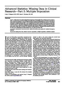
Multiple imputation (not to be confused with multiple consecutive layers of imputation) is a powerful technique which relies on taking multiple independent plausible imputed values for a missing value and combining them to find an improved imputation result (Schafer & Graham 2002). SiMI and the new technique k-Means SiMI both provide the ability to intuitively get such an imputation result. A decision forest (such as SysFor (Islam & Giggins 2011)) creates multiple trees based on considering different attributes as the root node and selecting different splitting points when generating the trees. If we consider each of the subsets found in these decision tree leaves to be a plausible subset for classifying a record, and instead perform EMI on the subset in order to impute missing values, then we create a system where we use several samples of the dataset to generate imputation results which should be close to the truth, as we already know that EMI performs better within the leaves of a decision tree (Rahman & Islam 2013b). Figure 5 provides an example of how a single record within a dataset of size n × m falls into a single leaf in a tree, but several in a forest. Each of the rectangular nodes represents a splitting point based
65
CRPIT Volume 168 - Data Mining and Analytics 2015
Figure 5: Example of leaves in a decision forest. on one of the m attributes in the dataset. The lines which proceed from these rectangular nodes explain the rules upon which the forest has split the data to create the subsets used in its child nodes. Circular nodes represent leaves, and the amount of records of each class that falls within each leaf is printed inside the node. The forest is built on the clean records of the dataset, of which there are 235 in this example. Let us assume that r1 has a missing value for attribute Aj . In order to impute the value for Aj , we first must see which leaf r1 falls into for each tree. In the figure, we see that record r1 falls into the middle leaf of T1 and leftmost leaf of T2 (this is indicated by the thick line linking the record to the leaves). We take the subset found from T1 containing 100 records, 80 of which are in class C1 and 20 of which are in class C2, and append our missing-value record r1 . With this subset we perform EMI to impute missing numerical attributes, and perform a mode imputation to impute missing categorical attributes. This gives us an im1 putation we store as rij , as this is the imputation for value ri j with the 1st tree. This process is repeated for each of the T trees in the forest. The second im2 putation rij will use a subset with 136 other records based on the leaf r1 falls into for T2 . In the process of modifying SiMI to use this technique we can skip the step of intersection, but still use SiMI’s merging strategy amongst the leaves of individual decision trees in order to ensure we have leaves
66
of sufficient size for our imputations. Each imputal tion for attribute Aj in ri can be represented as rij , and we express the full imputation as: T P
rij =
l rij
l=1
T
(6)
Making such a simple change may seem trivial, however the results speak for themselves (Figure 6). MultiSiMI (as we have dubbed this algorithm) outperforms SiMI on 6 of the 7 datasets we have presented. Of all the modification techniques attempted so far, it would appear that multiple imputation can provide the key to unlocking the potential of partition-discovering imputation techniques in the future. We can see in MultiSiMI the true potential for improvement that exists when making intelligent novel modifications to existing partition-discovering imputation algorithms. This technique could be applied to many other algorithms in both creative or trivial ways. An example of a trivial solution would be to perform a k-NN imputation multiple times with many k values, and average the results. 6
Conclusion
In this paper we have proposed a new technique based on combining a partition-discovering approach with
Proceedings of the 13-th Australasian Data Mining Conference (AusDM 2015), Sydney, Australia
Figure 6: MultiSiMI d2 results (higher the better) multiple imputation, discussed variants to partitiondiscovering algorithms and how they effect imputation accuracy, and classified several existing techniques into two classes: global and partitiondiscovering. We have thoroughly examined the innerworkings of some of these existing algorithms and shown through the development of our variants to SiMI and final proposed technique MultiSiMI how the process of making intelligent changes to existing missing value imputation algorithms provides grounds for future research and stronger imputation results. Our proposed algorithm, MultiSiMI, performs better than the original algorithms it is based on in six out of seven tested situations and is the major contribution of the paper. The others perform better on certain patterns of missingness, and particularly perform well on the AutoMPG dataset. A comprehensive analysis should be undertaken in the future to see what exactly makes these algorithms perform to a higher degree of success on particular datasets. The issue of parameters having a wildly unpredictable impact on decision tree based partition-discovering techniques is addressed and related to this issue. This is another potential field in which further research should be conducted. This paper achieves its aim of understanding the state of the art for missing value imputation and showing how that understanding can be translated
into successful new algorithms. By examining the impact on imputation accuracy caused by the proposed changes, we get an even better understanding of how the state of the art will change in the nearfuture. The process of data cleansing is essential in the field of data analysis, and so it is important that the processes used are practical and make use of the most appropriate techniques. We show how altering the method for partition-discovery in existing algorithms effects the imputation result through k-Means SiMI, show how using an early imputation step can be used to increase the quality of the final imputation result using EKSiMI, and explore the use of multiple imputation in order to remove any dependencies between consecutive imputation steps and find a higher quality overall imputation result, giving us our final proposed technique. The design philosophy for MultiSiMI can easily be translated to create many other novel techniques based on the multiple imputation paradigm. In many situations, it will be difficult to ascertain the correct parameters for missing value imputation algorithms, so we believe that an important step in the future is to develop techniques that require as little user input as possible. Complexity is also a major issue which is not addressed in many existing algorithms, with those algorithms instead being focussed on providing accuracy by any means necessary. Big data is said to consist of ”three v’s” - velocity, variety, and volume (Zikopoulos et al. 2011). The issue of complexity becomes increasingly important when we consider the volume of the data we are dealing with and the velocity at which it arrives - which of course requires it to be cleansed in a timely manner. None of the existing techniques discussed take this into serious account - so we see this as a strong contender for future research. The problem of missing values in datasets is by no means solved. Extensive changes to the field are expected to take place over the next few years, as better techniques are discovered and developed. This paper demonstrates the huge potential of the field’s future development and the practicality of employing these techniques. References Aydilek, I. B. & Arslan, A. (2013), ‘A hybrid method for imputation of missing values using optimized fuzzy c-means with support vector regression and a genetic algorithm’, Information Sciences 233, 25– 35. Bache, K. & Lichman, M. (2013), ‘UCI machine learning repository’. URL: http://archive.ics.uci.edu/ml Cai, Z., Heydari, M. & Lin, G. (2006), ‘Iterated local least squares microarray missing value imputation’, Journal of bioinformatics and computational biology 4(05), 935–957. Cheng, K.-O., Law, N.-F. & Siu, W.-C. (2012), ‘Iterative bicluster-based least square framework for estimation of missing values in microarray gene expression data’, Pattern recognition 45(4), 1281–1289. Dempster, A. P., Laird, N. M., Rubin, D. B. et al. (1977), ‘Maximum likelihood from incomplete data via the em algorithm’, Journal of the Royal statistical Society 39(1), 1–38. Islam, M. Z. & Giggins, H. (2011), Knowledge discovery through sysfor: a systematically developed
67
CRPIT Volume 168 - Data Mining and Analytics 2015
forest of multiple decision trees, in ‘Proceedings of the Ninth Australasian Data Mining ConferenceVolume 121’, Australian Computer Society, Inc., pp. 195–204. Jain, A. K. (2010), ‘Data clustering: 50 years beyond k-means’, Pattern Recognition Letters 31(8), 651– 666. Junninen, H., Niska, H., Tuppurainen, K., Ruuskanen, J. & Kolehmainen, M. (2004), ‘Methods for imputation of missing values in air quality data sets’, Atmospheric Environment 38(18), 2895– 2907. Mallinson, H. & Gammerman, A. (2003), ‘Imputation using support vector machines’. Nelwamondo, F. V., Mohamed, S. & Marwala, T. (2007), ‘Missing data: A comparison of neural network and expectation maximisation techniques’, arXiv preprint arXiv:0704.3474 . Quinlan, J. R. (1993), C4. 5: programs for machine learning, Vol. 1, Morgan kaufmann. Rahman, G. & Islam, M. Z. (2011), A decision tree-based missing value imputation technique for data pre-processing, in ‘Proceedings of the Ninth Australasian Data Mining Conference-Volume 121’, Australian Computer Society, Inc., pp. 41–50. Rahman, M. G. & Islam, M. Z. (2013a), ‘Missing value imputation using decision trees and decision forests by splitting and merging records: Two novel techniques’, Knowledge-Based Systems 53, 51–65. Rahman, M. G. & Islam, M. Z. (2013b), ‘A novel framework using two layers of missing value imputation’, Conferences in Research and Practice in Information Technology 146. Rahman, M. G. & Islam, M. Z. (2014), ‘Fimus: A framework for imputing missing values using coappearance, correlation and similarity analysis’, Knowledge-Based Systems 56, 311–327. Schafer, J. L. & Graham, J. W. (2002), ‘Missing data: our view of the state of the art.’, Psychological methods 7(2), 147. Schneider, T. (2001), ‘Analysis of incomplete climate data: Estimation of mean values and covariance matrices and imputation of missing values.’, Journal of Climate 14(5). Su, J. & Zhang, H. (2006), A fast decision tree learning algorithm, in ‘Proceedings of the National Conference on Artificial Intelligence’, Vol. 21, Menlo Park, CA; Cambridge, MA; London; AAAI Press; MIT Press; 1999, p. 500. Tresp, V., Neuneier, R. & Ahmad, S. (1995), Efficient methods for dealing with missing data in supervised learning, in ‘Advances in neural information processing systems’, MORGAN KAUFMANN PUBLISHERS, pp. 689–696. Troyanskaya, O., Cantor, M., Sherlock, G., Brown, P., Hastie, T., Tibshirani, R., Botstein, D. & Altman, R. B. (2001), ‘Missing value estimation methods for dna microarrays’, Bioinformatics 17(6), 520–525. Wang, Y., Wang, L., Yang, D. & Deng, M. (2014), ‘Imputing missing values for genetic interaction data’, Methods 67(3), 269–277.
68
Willmott, C. J. (1982), ‘Some comments on the evaluation of model performance’, Bulletin of the American Meteorological Society 63(11), 1309–1313. Xiang, Z. & Islam, M. Z. (2014), The performance of objective functions for clustering categorical data, in ‘Knowledge Management and Acquisition for Smart Systems and Services’, Springer, pp. 16–28. Zikopoulos, P., Eaton, C. et al. (2011), Understanding big data: Analytics for enterprise class hadoop and streaming data, McGraw-Hill Osborne Media.