Multiple Instance Learning for Classification of Human Behavior ...

Multiple Instance Learning for Classification of Human Behavior Observations Athanasios Katsamanis, James Gibson, Matthew P. Black, and Shrikanth Narayanan University of Southern California, http://sail.usc.edu

Abstract. Analysis of audiovisual human behavior observations is a common practice in behavioral sciences. It is generally carried through by expert annotators who are asked to evaluate several aspects of the observations along various dimensions. This can be a tedious task. We propose that automatic classification of behavioral patterns in this context can be viewed as a multiple instance learning problem. In this paper, we analyze a corpus of married couples interacting about a problem in their relationship. We extract features from both the audio and the transcriptions and apply the Diverse Density-Support Vector Machine framework. Apart from attaining classification on the expert annotations, this framework also allows us to estimate salient regions of the complex interaction. Keywords: multiple instance learning, support vector machines, machine learning, behavioral signal processing

1

Introduction

Behavioral observation is a common practice for researchers and practitioners in psychology, such as in the study of marital and family interactions [1]. The research and therapeutic paradigm in this domain often involves the collection and analysis of audiovisual observations from the subject(s) in focus, e.g., couples or families. Meticulous evaluation of these observations is critical in this context and is usually performed by carefully trained experts. Guidelines for this evaluation are typically provided in the form of coding manuals, which are often customized for a particular domain; for example, the Social Support Interaction Rating System (SSIRS) was created to code interactions between married couples [2]. These manuals aim at standardizing and expediting the coding process, which unfortunately can still remain laborious, resource-consuming, and inconsistent [1]. In our recent work [3, 4], we argued that the application of appropriate signal processing and machine learning techniques has the potential to both reduce the cost and increase the consistency of this coding process. We introduced a framework to automatically analyze interactions of married couples and extract audioderived behavioral cues. These low- and intermediate-level descriptors were then

2

A. Katsamanis, J. Gibson, M. Black, S. Narayanan

shown to be predictive of high-level behaviors as coded by trained evaluators. Building on this research, we are currently focusing on detecting salient portions of the voluminous, possibly redundant observations. This would enable us to better model the dynamics of the interaction by identifying regions of particular interest. In this direction, we formulate the automatic behavioral coding problem in a multiple instance learning setting and demonstrate the resulting benefits. Multiple instance learning (MIL), in machine learning terms, can be regarded as a generalized supervised learning paradigm, in which only sets of examples, and not single examples themselves, are associated with labels. The examples are referred to as “instances,” while the labeled sets are called “bags” [5]. Conventionally, a negatively labeled bag is assumed to contain only negative instances, while a positive bag should contain at least one positive instance. It is illustrative to consider the problem of object detection in images from this MIL perspective [6]. In most cases, image labels will only indicate whether an object exists or not in the image and will not provide information about its exact location. In MIL terminology, the image is the bag, and the various objects in the image are the instances. The image/bag will contain the requested object, i.e., be positively labeled, if at least one of the instances is indeed the requested object, i.e., is positive. Apart from object detection, MIL has been successfully applied in domains such as text and image classification [7–9], audio classification [10], and more recently in video analysis for action recognition [11]. In this paper, we argue that the MIL paradigm is well-suited for the automatic processing of behavioral observations, collected for the purpose of research in behavioral sciences like psychology. We properly adjust and employ the basic technique introduced in [8], which is known as Diverse Density Support Vector Machine and presented in detail in Sec. 2.2. In Sec. 2.3, we discuss the low-level lexical and intonation features that we extract from the corpus of married couple interactions (described in Sec. 2.1). In Sec. 3, we show significant improvement in predicting high-level behavioral codes using this MIL technique, which also has the advantage of simultaneously attaining saliency estimates for the observation sequences. We conclude in Sec. 4 with a discussion about ongoing work.

2 2.1

Proposed approach Corpus

Our current research focuses on a richly annotated audiovisual corpus that was collected as part of a longitudinal study on couple therapy at the University of California, Los Angeles and the University of Washington [12]. The study involved 134 seriously and chronically distressed married couples that received couple therapy for one year. The corpus comprises 574 ten-minute dyadic interactions (husband and wife), recorded at different times during the therapy period. During these sessions, the couple discussed a problem in their relationship with no therapist or research staff present. The recordings consist of a single channel of far-field audio and a split-screen video. No specific care was taken to

Human Behavior Multiple Instance Learning

3

standardize the recording conditions since the data were not intended for automatic processing. Word-level transcriptions for each session exist, which have allowed us to process the lexical content of the recordings without having to apply automatic speech recognition. A more detailed overview of the corpus can be found in [3]. For each session, both spouses were evaluated with 33 session-level codes from two coding manuals that were designed for this type of marital interaction. The Social Support Interaction Rating System (SSIRS) measures both the emotional features and the topic of the conversation [2]. The Couples Interaction Rating System (CIRS) was specifically designed for conversations involving a problem in the relationship [13]. Three to four trained evaluators coded each session, i.e., provided one set of 33 codes for each spouse, and all codes had written guidelines and were on an integer scale from 1 to 9. Due to low inter-evaluator agreement for some codes [3], we only chose to analyze the six codes with the highest inter-evaluator agreement (correlation coefficient higher than 0.7): level of blame and level of acceptance expressed from one spouse to the other (taken from the CIRS), global positive affect, global negative affect, level of sadness, and use of humor (taken from the SSIRS). Furthermore, similarly to what was done in our previous work [3], we framed the learning problem as a binary classification task. That is, we only analyzed sessions that had mean scores (averaging across evaluators) that fell in the top 25% and bottom 25% of the score range, i.e., approximately 180 sessions per code. In contrast with our previous studies, we select the extremely scored sessions in a gender-independent manner. The session-level code values are hereafter referred to as “low” and “high.” Thus, instead of trying to predict, for example, the numerical level of blame for a spouse in a given session, we are trying to predict whether the level of blame for that spouse is low or high. For this work, we will be using only observations from the coded spouse and not his/her partner. 2.2

MIL using Diverse Density SVMs

Diverse Density Support Vector Machines (DD-SVMs) were originally introduced for image retrieval and classification [8]. We discuss how this approach can also be of merit for the problem of automatic analysis of behavioral observations. Let B = {B1 , . . . , Bm } be the set of sessions and Y = {y1 , . . . , ym } be the corresponding set of session labels for one particular code; yi ∈ {−1, 1} is the ith session label (low or high). Based on the coding manuals [13, 2], session-level behavioral evaluation is based on the presence/absence of one or more events that occur during the interaction. For example, the level of sadness for a spouse may be judged as high if he/she cries, and the level of acceptance is low if the spouse is consistently critical. Here, we assume that each session can be represented as a set of behavioral events/instances, e.g., crying, saying “It’s your fault”. More formally, Bi = {Bi1 , . . . , BiNi }. Since we do not have explicitly labeled instances in our corpus, we need to come up with a method to label instances and determine their relevance with respect to the six codes we are analyzing.

4

A. Katsamanis, J. Gibson, M. Black, S. Narayanan

Diverse density to select instance prototypes In the MIL paradigm, one can intuitively expect that the instance labels can be found by exploiting the entire set of instances and labeled bags. This can be accomplished by comparing the frequency count of an instance across the low vs. high sessions. For example, an instance that only appears in low-blame sessions can reasonably be regarded as low-blame, while an instance that appears uniformly in all sessions cannot be regarded as blame-salient. In practice, given that each instance is represented by a noisy feature vector, the direct implementation of the above idea will typically lead to poor performance. In addition, one has to take into consideration the fact that an instance may not appear identically in two different bags. The so-called “diverse density,” which was introduced in [5], circumvents these difficulties by making proper assumptions on the probability distributions of both the instances and the bags. For a vector x in the instance feature space, diverse density is defined in [8] as:   Ni m Y Y 2  1 + yi − yi DD(x) = (1 − e−||Bij −x|| ) , (1) 2 i=1 j=1

where Bij is the feature vector corresponding to a certain instance. Instances that are close to instances in the high-rated sessions (yi = 1) and far from instances in the low-rated sessions (yi = −1) have a high diverse density and are assumed to be more salient for high values of the code. Following [8], we can then find local maxima of the diverse density function to identify the so-called instance prototypes, i.e., salient instances for each code. By reversing the yi labels, we can repeat the maximization process to identify the instance prototypes for the low values of each code. Distance metric to compute final features Having identified the set of instance prototypes {x∗1 , x∗2 . . . x∗M }, we can then represent each session Bi by a vector of distances from each prototype [8]:   minj ||Bij − x∗1 ||  minj ||Bij − x∗2 ||    d(Bi ) =  (2)  ..   . minj ||Bij − x∗M ||

Given this feature vector for each session, supervised classification can be performed using conventional SVMs. 2.3

Feature extraction

In this work, the instance was defined as a speaker turn, which simplified the fusion of lexical and audio features. We only used turns for which the temporal boundaries were reliably detected via a recursive speech-text alignment procedure [14].

Human Behavior Multiple Instance Learning

5

Lexical features Lexical information in each instance is represented by a vector of normalized products of term/word frequencies with inverse document frequencies (tfidf ) for a selected number of terms [15]. For a term tk that appears n times in the document dj , and in total appears in Dtk of the D documents, its tfidf value in dj is computed as follows [16]: tf idf (tk |dj ) =

(

n log

D−Dtk Dtk

0,

, Dtk 6= D Dtk = D

(3)

In order to account for varying turn lengths, we further normalize the tfidf values, so the feature vector has unit norm [15]: tf idf (tk |dj ) tf idfn (tk |dj ) = qP , W 2 tf idf (t |d ) s j s=1

(4)

where W is the number of turns in the instance. No stemming has been performed [15]. Term selection is achieved using the information gain, which has been found to perform better than other conventional feature selection techniques in text classification [17–19]. Information gain is a measure of the “usefulness”, from an information theoretic viewpoint, with regards to the discriminative power of a feature. For the binary classification case, i.e., classes c1 vs. c2 , the information gain G for a term tk can be estimated as follows [17]: G(tk ) = − + P r(tk )

2 X

i=1 2 X i=1

P r(ci ) log P r(ci ) P r(ci |tk ) log P r(ci |tk ) + P r(t¯k )

2 X

P r(ci |t¯k ) log P r(ci |t¯k ),

(5)

i=1

where t¯k represents the absence of the term tk . Terms with lower information gain than a minimum threshold were ignored. The minimum threshold was set so that only 1% of the terms were kept. The first 10 selected terms for the whole corpus are given in Table 1, sorted by decreasing information gain for each behavior. Interestingly, fillers like “UM” and “MM” and “(LAUGH)” appear to have significant information gain for more than one behaviors. Audio features For the representation of intonation extracted from the audio, we use a codebook-based approach. Intonation information in each turn is represented by a vector of normalized frequencies of “intonation” terms. These terms are defined by means of a pitch codebook. This is built on sequences of pitch values. Given the highly variable audio recording conditions and speaking styles, the codebook allows us to filter our data and only account for prototypical intonation patterns. The audio feature extraction algorithm mainly involves three steps:

6

A. Katsamanis, J. Gibson, M. Black, S. Narayanan Behavior

Informative words

acceptance UM, TOLD, NOTHING, MM, YES, EVERYTHING, ASK, MORE, (LAUGH), CAN’T blame NOTHING, EVERYTHING, YOUR, NO, SAID, ALWAYS, CAN’T, NEVER, MM, TOLD humor (LAUGH), TOPIC, GOOD, MISSING, COOL, TREAT, SEEMED, TRULY, ACCEPT, CASE negative TOLD, KIND, MM, MAYBE, NOTHING, UM, YOUR, NEVER, CAN’T, (LAUGH) positive UM, KIND, NOTHING, MM, GOOD, (LAUGH), TOLD, CAN’T, MEAN, WHY sadness ACTUALLY, ONCE, WEEK, GO, OKAY, STAND, CONSTANTLY, UP, ALREADY, WENT Table 1. Terms with the highest information gain for discriminating between extreme behaviors.

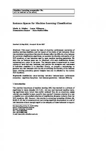
1. Pitch and intensity estimation Raw pitch values are extracted from the audio as described in [3] every 10ms. Non-speech segments are excluded by applying voice activity detection [20]. Pitch values are automatically corrected for spurious pitch-halving or doubling, and are then median-filtered and interpolated across unvoiced regions. Finally, pitch f0 measurements are speaker-normalized [3], i.e., fˆ0 = f0 − f0µ , where f0µ is the mean speaker pitch, estimated over the whole session. 2. Resampling and buffering The pitch signals are low-pass filtered and resampled at 10Hz, i.e., we get one pitch value every 100ms. Each of these values roughly corresponds to the duration of a single phoneme. Since we expect informative intonation patterns to appear in a longer duration, approximately equal to the duration of at least two words, we group sequential values of pitch inside a window of 1sec duration, to create 10-sample pitch sequences. The window is shifted every 100ms. 3. Clustering and counting We cluster the resulting sequences using K-means. Each sequence is then represented by the center of the cluster in which it belongs. In analogy with the text representation, we consider the pitch cluster centers to be our intonation terms and we estimate their frequency of appearance in each turn. The five most frequent occuring intonation terms are shown in Fig. 1.

3

Experiments

We compare the classification performance of the proposed approach with a conventional SVM-based classification scheme. All our experiments are performed using 10-fold cross-validation. The folds were determined in the set of couples

Human Behavior Multiple Instance Learning

7

Frequently appearing intonation terms 40

20

Hz

0

−20

−40 26%

−60

0.2

24%

0.4

10%

0.6 sec

8%

8%

0.8

1

Fig. 1. The five most frequently appearing intonation terms are shown. Each term is defined as one of the 10 cluster centers to which 1-s long pitch sequence observations were clustered using k-means. The appearance frequency of each term is given as a percentage of the total number of pitch sequence observations.

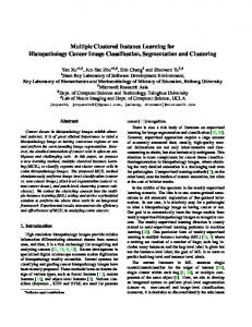
and not in the set of sessions. In this way, we did not have any folds where a session from a training couple would appear in the testing set. Binary classification, i.e., “high” vs. “low”, accuracy results are given as box plots in Fig. 2 for three cases, namely when using lexical features with a standard SVM, when using lexical features in the multiple instance learning scheme described earlier and when intonation features are also used in the same setup. Lexical and intonation features are extracted as described in Sec. 2.3. The leftmost box in each graph corresponds to the baseline, i.e., the standard SVM-based approach. The central line on each box is the median, while the diamonds represent the mean values. For the conventional SVM the session features were extracted over the whole session and not separately for each speaker turn. Based on the mean values and the overall distribution of the results for the 10 folds, there are two things that can be noted, namely overall performance is improved when switching to the MIL setup and the intonation features do not lead to further consistent accuracy improvements.

8

4

A. Katsamanis, J. Gibson, M. Black, S. Narayanan

Conclusions and future work

We showed that the Multipe Instance Learning framework can be very useful for the automatic analysis of human behavioral observations. Our research focuses on a corpus of audiovisual recordings of marital interactions. Each interaction session is expected to comprise multiple instances of behavioral patterns not all of which are informative for the overall session-level behavioral evaluation of an interacting spouse. By means of the so-called diverse density we are able to identify salient instances that have significant discriminative power. Saliency is defined with reference to a specific discrimination task each time. We demonstrated improved performance when classification was only based on these salient instances. In the future, we plan to further elaborate on the saliency estimation aspect of the proposed approach. Further, we would like to investigate alternative intonation and, in general, audio-based features that would help us more effectively exploit the corresponding information in the proposed scheme.

5

Acknowledgements

We are grateful to Brian Baucom and Andrew Christensen for giving us access to the couple therapy dataset. This research is partially supported from the National Science Foundation.

References 1. G. Margolin, P.H. Oliver, E.B. Gordis, H.G. O’Hearn, A.M. Medina, C.M. Ghosh, and L. Morland, “The nuts and bolts of behavioral observation of marital and family interaction,” Clinical Child and Family Psychology Review, vol. 1, no. 4, pp. 195–213, 1998. 2. J. Jones and A. Christensen, Couples interaction study: Social support interaction rating system, University of California, Los Angeles, 1998. 3. M. P. Black, A. Katsamanis, C.-C. Lee, A. C. Lammert, B. R. Baucom, A. Christensen, P. G. Georgiou, and S. Narayanan, “Automatic classification of married couples’ behavior using audio features,” in Proc. Int’l Conf. on Speech Communication and Technology, 2010. 4. C.-C. Lee, M. P. Black, A. Katsamanis, A. C. Lammert, B. R. Baucom, A. Christensen, P. G. Georgiou, and S. Narayanan, “Quantification of prosodic entrainment in affective spontaneous spoken interactions of married couples,” in Proc. Int’l Conf. on Speech Communication and Technology, 2010. 5. O. Maron and T. Lozano-P´erez, “A framework for multiple instance learning,” in Proc. Advances in Neural Information Processing Systems, 1998. 6. P. Viola, J. C. Platt, and C. Zhang, “Multiple instance boosting for object detection,” in Proc. Advances in Neural Information Processing Systems, 2006. 7. S. Andrews, I. Tsochantaridis, and T. Hofmann, “Support vector machines for multiple instance learning,” in Proc. Advances in Neural Information Processing Systems, 2003.

Human Behavior Multiple Instance Learning

9

8. Y. Chen and J. Z. Wang, “Image categorization by learning and reasoning with regions,” Journal of Machine Learning Research, vol. 5, pp. 913–939, 2004. 9. Y. Chen, J. Bi, and J. Z. Wang, “MILES: Multiple instance learning via embedded instance selection,” IEEE Trans. Pattern Anal. Mach. Intell., vol. 28, pp. 1931– 1947, 2006. 10. K. Lee, D. P. W. Ellis, and A. C. Loui, “Detecting local semantic concepts in environmental sounds using Markov model based clustering,” in Proc. IEEE Int’l Conf. Acous., Speech, and Signal Processing, 2010. 11. S. Satkin and M. Hebert, “Modeling the temporal extent of actions,” in Proc. European Conf. on Computer Vision, 2010. 12. A. Christensen, D.C. Atkins, S. Berns, J. Wheeler, D.H. Baucom, and L.E. Simpson, “Traditional versus integrative behavioral couple therapy for significantly and chronically distressed married couples,” Journal of Consulting and Clinical Psychology, vol. 72, no. 2, pp. 176–191, 2004. 13. C. Heavey, D. Gill, and A. Christensen, Couples interaction rating system 2 (CIRS2), University of California, Los Angeles, 2002. 14. A. Katsamanis, M. Black, P. Georgiou, L. Goldstein, and S. Narayanan, “SailAlign: Robust long speech-text alignment,” in Workshop on New Tools and Methods for Very-Large Scale Phonetics Research, 2011. 15. F. Sebastiani, “Machine learning in automated text categorization,” ACM Computing Surveys, vol. 34, pp. 1–47, 2002. 16. G. Salton and C. Buckley, “Term-weighting approaches in automatic text retrieval,” Information Processing and Management, vol. 24, pp. 513–523, 1988. 17. Y. Yang and J. O. Pedersen, “A comparative study on feature selection in text categorization,” in Proc. Int’l Conf. on Machine Learning, 1997. 18. G. Forman, “An extensive empirical study of feature selection metrics for text classification,” Journal of Machine Learning Research, vol. 3, pp. 1289–1305, 2003. 19. E. Gabrilovich and S. Markovitch, “Text categorization with many redundant features: using aggressive feature selection to make SVMs competitive with C4.5,” in Proc. Int’l Conf. on Machine Learning, 2004. 20. P. K. Ghosh, A. Tsiartas, and S. S. Narayanan, “Robust voice activity detection using long-term signal variability,” IEEE Trans. Audio, Speech, and Language Processing, 2010, accepted.

10

A. Katsamanis, J. Gibson, M. Black, S. Narayanan

1

1 0.95

0.95 accuracy

accuracy

0.9 0.9 0.85 0.8

0.85 0.8 0.75 0.7

0.75

0.65 acceptance

blame

1

lexical (SVM)

0.95

0.8

0.9

0.7

0.85

accuracy

accuracy

0.9

0.6 0.5

0.8

lexical (MIL)

0.75 lexical + intonation (MIL)

0.7 0.65

0.4

0.6 humor

negative

0.95

1

0.9 0.85 accuracy

accuracy

0.95

0.9

0.8 0.75 0.7

0.85

0.65 positive

sadness

Fig. 2. Binary 10-fold cross-validated classification results for lexical and audio feature sets using conventional SVMs or Diverse Density SVMs for six behavioral codes. The central line on each box is the median, while the edges are the 25th and 75th percentiles. The diamonds correspond to the mean values. The whiskers extend to the most extreme fold accuracy values which are not considered outliers. Points that are smaller than q1 − 1.5(q3 − q1 ) or greater than q3 + 1.5(q3 − q1 ), where q1 and q3 are the 25th and 75th percentiles respectively, are considered to be outliers and are marked with crosses. The leftmost box in each graph corresponds to the conventional SVM classification with lexical features while the central and rightmost boxes illustrate the results of the MIL approach with lexical features only and joint lexical and intonation features respectively.