Multiple Instance Learning for Malware Classification - arXiv

1

Multiple Instance Learning for Malware Classification

arXiv:1705.02268v1 [cs.CR] 5 May 2017

Jan Stiborek, Tomáš Pevný, Martin Rehák

Abstract—This work addresses classification of unknown binaries executed in sandbox by modeling their interaction with system resources (files, mutexes, registry keys and communication with servers over the network) and error messages provided by the operating system, using vocabulary-based method from the multiple instance learning paradigm. It introduces similarities suitable for individual resource types that combined with an approximative clustering method efficiently group the system resources and define features directly from data. This approach effectively removes randomization often employed by malware authors and projects samples into low-dimensional feature space suitable for common classifiers. An extensive comparison to the state of the art on a large corpus of binaries demonstrates that the proposed solution achieves superior results using only a fraction of training samples. Moreover, it makes use of a source of information different than most of the prior art, which increases the diversity of tools detecting the malware, hence making detection evasion more difficult. Index Terms—Malware, dynamic analysis, sandboxing, multiple instance learning, classification, random forest.

I. M OTIVATION Since malware is presently one of the most serious threats to computer security with the number of new samples reaching 140 million in 2015 [3], battles against it are fought on many fronts. Signature matching remains the core defense technology, but due to evasion techniques such as polymorphism, obfuscation, and encryption, keeping good recall is difficult for static analysis and methods based purely on string matching. A popular approach to tackle these problems is to execute a binary in a controlled environment (sandbox) [35], monitor its behavior, and based on this behavior classify the sample into benign or malware class (or as a particular malware family). The assumption of these dynamic analysis methods is that behavior should be more difficult to randomize and therefore it should constitute a more robust signal. Most approaches to dynamic analysis rely on system calls [32], [1], [45], as they are the only means how the binary can interact with the operating system and other resources. This popularity has however already triggered many evasion techniques, such as shadow attacks [29], system-call injection attacks [22], or sandbox detection [16]. A perpendicular approach to modeling system calls is to model resources the binary has interacted with together with the type of the resources. The rationale is that if malware wants to provide revenue to its owner, it has to perform actions, such as downloading advertisements in the case of adware, encrypting hard drive in the case of ransomware, exfiltrating sensitive data in the case of credential stealers, etc. This work assumes that execution of these actions involves interactions

with resources visible at the operating system level, and this interaction can be viewed as a signal which is hard to hide and which can be indicative of malware families. Modeling interactions with system resources has been already exploited by the prior art. Mohaisen et al. [30] extracts a manually predefined set of features such as number of files created in specific folders, number of HTTP requests, etc., and use it in supervised classification. However, we believe that the rapidly changing threat landscape makes it difficult to manually design features that are indicative while also being stable over time. An alternative paradigm is to avoid manual design and to use a bag-of-words model (BoW model), where every interaction with a particular resource identified by its name is considered as a unique feature [38]. The price paid for circumventing manual feature design using BoW is an explosion of the problem dimension, which can easily reach millions. This work circumvents the problem of manually designing features while at the same time avoiding the problem dimension explosion. The approach is to first cluster resource names with similarity functions tailored for each resource type (file names, mutexes, registry names, and domain names), and then use this clustering to represent a sample (a binary executed in the sandbox) in a lower-dimensional space. This enables us to use a random forest classifier (or any other classifier of choice) to separate malware from legitimate samples. The clustering also effectively removes randomization used to evade detection. The proposed approach is extensively evaluated on a large number of samples (more than 200 000) and compared to relevant prior art. Experimental results show that the proposed approach indeed improves the accuracy of detecting malware binaries. The contributions of this paper are manifold including a novel approach to representing malware using raw data, definition of a similarity measure reflecting directory structure, optimization of similarity function over binaries, improvements to Louvain clustering in order to scale to large scale datasets, and finally evaluation and comparison to state-ofthe-art approaches on real-world malware using large-scale dataset. II. C LASSIFICATION OF SANDBOXED SAMPLES To capture the malware behavior, this work assumes that execution of malware’s actions involves interactions with resources visible at the operating system level. Examples of such interactions include operations with files during encryption of a victim’s hard drive, network communication during

2

data exfiltration or displaying advertisements, operation with mutexes used to ensure a single instance of malware is running, or manipulation with registry keys to ensure persistency after reboot. An additional source of information are error messages of the operating system itself. Such information is provided by the sandboxing environment as the following warnings: dll not found indicating missing dynamic library, incorrect executable checksum indicating corrupted binary, and sample did not execute indicating the fact that the binary was not executed at all due to various reasons (corrupted binary, sandbox was not able to copy the binary into VM, etc). To model the interactions of a malware binary with resources, this work views each binary executed in a sandbox as a set of pairs of names and types of resources the binary interacted with. This view frames the problem as a multiple instance learning (MIL) problem where each sample (binary) consists of a set of instances of different size. In our scenario an instance represents the pair of name and type of a resource the binary interacted with during sandboxing. Algorithm 1 High-level overview of training (function TRAIN) and classification (function PREDICT) of malware samples. 1: function TRAIN (S, y) ⊲ Training samples and labels 2: I ← extractInstances(S) 3: C ← cluster(I) ⊲ Clustering of instances (separately for individual types) 4: X ← project(S, C) ⊲ Projection of samples into binary vector (Alg. 2) 5: M ← trainClassifier(X, y) 6: return M, C ⊲ Returns cluster centers C and trained classifier M 7: end function 8: function PREDICT (S ′ , C, M)⊲ Testing samples S ′ , clusters C and classifier M 9: X ′ ← project(S ′ , C) ⊲ Projection of samples into binary vector (Alg. 2) 10: yˆ ← predict(M, X ′ ) ⊲ Classification of testing samples 11: return yˆ 12: end function Variable sizes of samples and lack of order over their instances pose a challenge to traditional machine learning methods that expect samples to have fixed size. A recent review of MIL algorithms [2] lists various approaches to overcome this variability in sample sizes. One of the most popular (also adopted in this work) is vocabulary-based method outlined in Algorithm 1. It employs clustering of instances to describe the sample by a fixed-dimensional vector with length equal to the size of vocabulary, i.e. a set of clusters, so that an ordinary machine learning method can be applied. To convert a sample into a fixed-dimensional vector, all instances I from all training samples S are extracted and clustered by a suitable method per given resource type–files, mutexes, registry keys, network communication. Note that warnings generated by the sandboxing environment are used

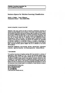
Algorithm 2 Projection of samples S into binary vector using cluster centers C. 1: function PROJECT (S, C) ⊲ Samples S and clusters C. 2: X ←∅ 3: for all s ∈ S do 4: I ← extractInstances(s) 5: x ← ~0 6: for all i ∈ I do 7: c∗ ← nnSearch(i, C) ⊲ Finds closest center c∗ to instance i. ∗ 8: x[c ] ← 1 9: end for 10: X ← X ∪ {x} 11: end for 12: return X 13: end function Binary 1

Binary 2

\Temp\4ffdd6ab-8020\config.dmc \Temp\4ffdd6ab-8020\bin.dmc \Windows\System32\ftp.exe

\Temp\ed8a9718-c7a0\config.dmc \Temp\ed8a9718-c7a0\bin.dmc \Windows\System32\netsh.exe

(a) raw filenames Binary 1

Binary 2

Artifact cluster 1 Artifact cluster 1 Artifact cluster 2

Artifact cluster 1 Artifact cluster 1 Artifact cluster 2

(b) artifact clusters

Table I: Example of clustering files of two binaries from the same family executed in the sandbox. directly, i.e. every warning is considered as a separated cluster. The resulting clusters represent the vocabulary. Next, for every instance i the closest cluster prototype c∗ (a small random subset of the cluster of instances) of corresponding type is located. Finally, the binary representation is then used such that element of the vector equals to 1 iff there was an instance close to the particular cluster prototype. Once all samples are encoded as fixed-dimensional vectors, one can use a machine learning algorithm of choice to implement the classifier. This work uses the random forest classifier [8] due to its versatility, accuracy, and scalability, which make it a popular choice for many different machine learning tasks including malware classification [17]. Since the clustering is an essential component of the above algorithm, the definition of similarity over instances (resource names) greatly influences the accuracy of the system, and therefore it should reflect properties of the application domain. The rest of this section defines a specific similarity metric for each type of resources the malware interact with, namely on files, mutexes, network hostnames, and registry keys, and also justifies our choice of the clustering method. A. Similarity between file paths Although viewing file paths as strings would allow to use vast prior art such as Levenshtein distance [25],

3

Hamming distance, Jaro-Winkler distance [33], or string kernels introduced in [28], the file systems were designed as tree structures with names of some folders (fragments of the path) being imposed by the operating system and the distance should reflect that. For example two files with paths /Documents and Settings/Admin/Start Menu/Programs/Startup/tii9fwliiv.lnk and /Documents and Settings/Admin/Start Menu/Programs/Accessories/Notepad.lnk share large parts of their paths and common string similarities will return high similarity score, but they serve very different purposes, since the first file is a link to an application executed after the start of the operating system (OS), while the second is a regular link in the Start menu in Windows OS. Another aspect that prohibits the use of common string similarities is their computational complexity (typically O(n2 ) where n is the length of the string). The complexity combined with the number of resources to be clustered (in order of millions) leads to unfeasible time requirements. This motivates the design of a similarity that is fast and takes into the account the tree structure of the file system, special folders, and differences between folders and filenames. The proposed similarity s(x, x′ ) of two file paths x and x′ is defined as
s(x, x′ ) = exp −wT f (x, x′ ) ,

(1)

where w is a vector of weights and f (x, x′ ) is a function extracting a feature vector from file paths x and x′ . Both the weight vector w and function f play an essential role and are both discussed in detail below. The function f in (1) captures differences between the two paths x and x′ by a fixed-dimensional vector. It first splits both paths x and x′ into fragments xi and x′i using OS specific path separator1 , in the cases of MacOS and Windows changes all characters to lowercase, and assigns all fragments into one of the following four categories: 1) known folder – fragment xi is a well known folder in the list of folders imposed by the operation system (e.g. Windows, Program Files, System32, etc.), 2) general folder – fragment xi is a not-well-known folder (e.g. unknown folders in Program Files, randomly generated folders in Internet Explorer cache folder, etc.), 3) file – fragment xi is file, 4) empty – artificial fragment used for padding the paths in cases when paths x and x′ have different depths. When all fragments are assigned to one of the above classes, their dissimilarity is captured by the function f as f (x, x′ ) = (fKK , fKG , fKF , fKE , fGG , fGF , fGE , fF F , fF E ) where • fKK is the number of fragments on the same level that were both classified as known folder and were not equal, • fGG is the sum of Levenshtein distances between all fragments on the same level that were classified as general folder, 1 Unixes

and MacOS uses ’/’ as a path separator, Windows uses ’\’.

•

•

fF F is the sum of Levenshtein distances of all fragments on the same level that were classified as file, fKG , fKF , fKE , fGF , fGE , fF E are the sums of all fragments of the same level and were classified as known and general folder, known folder and file, known folder and empty, general folder and file, general folder and empty, and file and empty respectively.

To illustrate the calculation of f (x, x′ ), let’s consider the same two paths used above. At first, function f splits both paths into fragments and assign them into one of four categories (see Table II). Assigning fragment to classes requires a list of known folders2 , which for the purpose of this example we assume to contain Documents and Settings, Start Menu, Programs and Startup, which are present in all windows installations. All corresponding folders from those two paths are therefore assigned to known folder class, while Admin and Accessories are labeled as general folders.3 Individual elements of the vector f (x, x′ ) are calculated using the above rules as follows: the first rule applies to three fragments 1, 3, and 4 belonging to known folder class, but as they are all equal fKK = 0; the second rule returns 0 based on analogous reasoning but for general folders; the third rule returns fF F = 0.7143, which is the Levenshtein distance between tii9fwliiv.lnk and Notepad.lnk; the only mismatch is on fragment 5–known folder and general folder yielding fKG = 1; and finally all remaining elements of feature vector are 0. The output of f (x, x′ ) is captured by the feature vector f (x, x′ ) = (0, 0, 0.7143, 1, 0, 0, 0, 0, 0). The weight vector w in (1) captures the contribution of individual elements of the feature vector f (x, x′ ). Imposing condition w ≥ 0, in combination with construction of function f , bounds the value of the similarity function (1) s(x, x′ ) ∈ [0, 1] such that the similarity functions returns 1 (or values close to 1) if x and x′ belong to the same class (files in /temp/ directory, cache of the Internet Explorer, files in system directory, etc.) and values approaching 0 if they belong to different classes. Since the similarity function (1) was inspired by the popular Gaussian kernel, the parameter vector w was optimized using the Centered Kernel Target Alignment [10] (CKTA), which is a method to optimize kernel parameters. CKTA assumes training data {(xi , yi ), }m i=1 where xi is a file path and yi is the class of the path xi , and defines centered kernel matrix as

w [Sw c ]ij = Sij −

m m m 1 X w 1 X w 1 X w Sij − Sij + 2 S , (2) m i=1 m j=1 m i,j=1 ij

2 Full list of known folders is available online: https://github.com/SfinxCZ/Malware-analysis-using-multiple-instancelearning 3 The first three known folders are embedded in the functionality of the Windows OS. The Startup folder has a specific meaning altering the behavior of the operation system since all programs listed in this folder are executed after the boot of the OS. On the other hand Accessories can be easily changed without major consequences.

4

x x′

Fragment 1

Fragment 2

Fragment 3

Fragment 4

Fragment 5

Fragment 6

Documents and Settings (K) Documents and Settings (K)

Admin (G) Admin (G)

Start Menu (K) Start Menu (K)

Programs (K) Programs (K)

Startup (K) Accessories (G)

tii9fwliiv.lnk (F ) Notepad.lnk (F )

Table II: Example of two paths x and x′ separated into individual fragments with labels (K – known folder, G – general folder and F – file). where Sw ij = sw (xi , xj ) is the kernel matrix corresponding to the similarity function (1) parametrized by the weight vector w. CKTA maximizes correlation between labels and a similarity matrix by solving the following optimization problem w∗ = arg max w≥0

hSw c , Y c iF , w kSc kF · kYc kF

(3)

where Y is target label kernel with [Y]ij equals to 1 when ith and j th paths from training data belongs to the same class and −1 otherwise, h·, ·iF is Frobenius product and k·kF is Frobenius norm (see Appendix A for more details). In below experiments (3) is solved by stochastic gradient descent (SGD) algorithm [6]. Note that although the path similarity s(xi , xj ) is not a valid kernel because it is not positive definite, the use of centered kernel alignment is still possible as the only limitation is that the global optimum might not be found. To finish the example, the similarity function (1) with weight vector w = (2, 10−5 , 1, 2.3, 1.6, 1, 0.36, 0.7, 0.9) returns the value s(x, x′ ) = 0.049, which correctly indicates that the two paths are different. B. Similarity of network traffic To define the similarity between network resources one has to overcome the randomization often employed by malware authors that render trivial similarity based on names of network resources (domains, IPs) ineffective. To escape blacklisting command and control (C&C) channels of malware, its authors use various techniques to hide and obscure C&C operation. Popular approaches include randomization of domain names by generating them randomly (DGA), quickly changing hosting servers and / or domain names by fast flux, or using large hosting providers like Amazon Web Services to hide among legitimate servers, etc. These techniques are relatively cheap (e.g. registering a new .com domain costs ~3USD per 1 year) and they allow for variation in domain names without updating disseminated malware binaries. In contrast, switching from one C&C paradigm to another requires such an update and therefore occurs relatively infrequently. These two properties contribute to each malware family using specific patterns of domain names, paths, and parts of URLs. Exploiting these patterns allows to group domain names into clusters. In this work the similarity in network traffic is defined only for HTTP/HTTPS protocol, because it is presently the default choice for malware authors as it is rarely filtered. The extension to other network traffic is possible [23]. The similarity in URL patterns used in this work has been adopted from [21], which has proposed to cluster domain names so that each cluster contains domains of one type / for one family of malware. The calculation of similarity starts by

grouping all HTTP/HTTPS requests using the domain names. Then the model of each domain name is built from path and query strings, transferred bytes, duration of requests and interarrival times (time spans between requests to the same domain) of individual requests to it. Finally, these models are used to calculate the similarity function between two domain names in the clustering. Since the calculation of the similarity is out of scope, we refer to an original publication [21] for details. C. Similarity between mutex names Mutex (Mutual exclusive object) is a service provided by most modern operating systems to synchronize multi-threaded and multi-processes applications. This mechanism is popular among malware authors to prevent multiple infections of the same machine, because running two instances of the same malware can cause conflicts limiting the potential revenue. Mutexes are identified by their name, which can be an arbitrary string. The naming scheme is challenging for malware authors, because the names cannot be static, which would make them good indicators of compromise of a particular malware, but they cannot be completely random either, because two independent binaries of the same family would not be able to check the presence of each other. Therefore malware authors resorted to pseudo-deterministic algorithms or patterns for generating mutex names. For some malware families these patterns are already well known, for example Sality [43] uses mutex names of the form ".exeM__"-explorer.exeM_1423_. Since operating systems do not impose any restrictions on the names of mutexes, they can be arbitrary strings. Therefore standard string similarities such as Levenshtein distance, Hamming distance, Jaro-Winkler distance, etc. can be used. In experiments presented in Sections III Levenshtein was used, as it gives overall good results. D. Similarity between registry names In Microsoft Windows operating system, the primary target of the majority of malware, registry serves as a place where programs can store various configuration data. It is a replacement of configuration files with several improvements such as strongly typed values, faster parsing, ability to store binary data, etc. The registry is a key-value store, where key names have the structure of a file system. The root keys are HKEY_LOCAL_MACHINE, HKEY_CURRENT_USER, HKEY_CURRENT_CONFIG, HKEY_CLASSES_ROOT, HKEY_USERS and HKEY_PERFORMANCE_DATA; some root keys also always have sub-keys with specific names (Software, Microsoft, Windows, etc.). Due to similarity with a file system, the similarity distance is the same as the one defined in Subsection II-A, but with a different set of

5

names of known folders and a weight vector optimized on registry data rather than on files. E. Clustering of resource names The above similarities are not true distances, which limits the choice of applicable clustering methods to those that do not require proper distance metric between points. The Louvain method [7] is a popular choice and it is used in experiments below, because it also automatically determines the number of clusters and thus removes the need to set it manually. The use of the Louvain method is the authors’ preference, but other clustering methods can be used as well; the reader is referred to [15] for an overview of methods requiring only similarity. Algorithm 3 Approximative clustering algorithm for instances I (resource names). 1: function APPROX C LUSTER(I; k, m, ǫ) 2: C=∅ 3: while I 6= ∅ do 4: I ′ ← Random subset of size k from I 5: C ′ ← cluster(I ′ , m) ⊲ Cluster instances I ′ and create cluster prot. of size m. 6: for all i ∈ I \ I ′ do 7: c∗ ← nnSearch(i, C ′ ) ⊲ Find cluster prot. c∗ closest to instance i. 8: if s(i, c∗ ) > ǫ then 9: c∗ ← c∗ ∪ {i} 10: end if 11: end for 12: C ← C ∪ C′ 13: end while 14: return C 15: end function The use of the Louvain method is not straightforward in the scenario of this paper because it requires a full adjacency matrix in advance. This results in a lower bound to computational complexity being O(n2 ) in the number of resources, which is clearly prohibitive as the number of unique resource names to cluster can easily reach the order of millions. To decrease the number of calculated similarities, an approach inspired by [46], [47], [20] is adopted where the Louvain clustering is used iteratively as summarized in Algorithm 3. Given a set of instances I of a particular type, in every iteration the algorithm selects a random subset I ′ ⊂ I of the data of size k small enough for the Louvain method to be computationally feasible. The results of the Louvaine clustering are then transformed to cluster prototypes—random subsets of clusters with size limited to m. Remaining data I\I ′ are then traversed and all samples with similarity larger than ǫ to some cluster prototype c∗ ∈ C ′ are added to c∗ and removed from I. Finally, C ′ is merged with the clustering C obtained in the previous iteration, and if I is not empty, the process is repeated. Clearly the algorithm is an approximation of a clustering with complete data and its performance depends on the choice of parameters k and ǫ. Experiments indicate that if

parameter k is large enough (k = 105 ) and parameter ǫ is set reasonably (in the experimental evaluation we use ǫ = 0.4, see Section III-B for details), the results are comparable with clustering methods applied to the complete data. The computational complexity of this sequential approximation is O (l · (k · (k − 1) /2 + cl · m · (nl − k))) where l is the number of iterations of algorithm (typically l ≤ 10), nl is the number of non-clustered samples in l-th iteration, k is the number of randomly selected samples, cl is the number of cluster prototypes produced by the clustering algorithm in lth iteration and m is the maximal size of a cluster prototype (typically m = 10). Since the parameter k is fixed and k ≪ n, we can see that the number of evaluations of the similarity function is linear in the number of samples, which clearly outperforms the quadratic complexity required by the vanilla Louvain method. III. E VALUATION In this section the proposed approach is compared to the approach proposed by Rieck, et al. [38] (further referred to as Rieck) and the approach proposed by Mohaisen, et al. [30] (further referred to as AMAL). Rieck has been selected as a representative of the prior art that encodes malware behavior into a high-dimensional feature space using bag-ofwords model built directly from data; it uses kernelized SVM to classify binaries. The second approach, AMAL, encodes malware behavior using a relatively low number of handmade features; to classify unknown binaries AMAL trains multiple classifiers (SVM, decision trees, k-nearest neighbor, etc.) and selects the optimal classifier for given data using cross-validation. A. Data set description The dataset used for experiments contained 250 527 files collected from October 24, 2016 to December 12, 2016 using AMP ThreatGrid [18]. All files were also analyzed by VirusTotal.com service [19] and labeled using its verdicts as follows: a file was labeled as malicious if at least 4 out of 10 selected AV engines (see Table IV for details) detected the file as malicious, and it was labeled as legitimate if none of the AV engines detected the file. Remaining files were discarded as unknown and removed from both training and testing sets in order to limit the effect of misclassifications by individual AV engines. The final numbers of files were: 144 229 malicious, 87 026 legitimate, and 19 272 discarded as unknown. The numbers of samples of individual malware families are summarized in Table III. All files were executed in sandbox by AMP ThreatGrid [18] service, using Windows 7 64bit (71% samples) environment, as it is the most popular OS at the time of writing4 , and Windows XP (29% samples) environment, since it is still widely deployed on embedded machines such as ATMs. Virtual machines were connected to the Internet without any filtering or restrictions that could by any mean prevent connections to 4 According to http://www.w3schools.com/browsers/browsers_os.asp Windows 7 has 34.6% market share against 1.0% covered by Windows XP, 11.1% covered by Windows 8 and 30.9% covered by Windows 10.

6

Malware family nemucod cerber bladabindi locky gamarue darkkomet hupigon upatre tinba scar swrort zbot virlock fareit farfli zegost virut adwind zusy ircbot zerber palevo vobfus delf donoff

#samples 13 781 12 829 10 945 9894 7694 4664 3555 3269 3104 2961 2868 2426 1797 1763 1749 1719 1556 1537 1505 1447 1329 1270 1244 1228 1211

Malware family amonetize nanocore loadmoney yakes bifrose autoit kolabc waldek pdfka shipup rebhip razy agentb poison xtrat onlinegames ramnit magania atraps softpulse banload ruskill downloadassistant binder remaining MW families

#samples 1172 1032 964 892 804 781 707 686 649 625 613 599 579 551 511 502 493 463 461 460 387 374 373 350 31 856

Total malicious

144 229

Total legitimate

87 026

Table III: Number of samples of malware families in the data set. The malware families for individual samples were determined using AVClass tool [40]. AhnLab, V3 Internet Security Avira, Antivirus Pro Bitdefender, Internet Security ESET, Internet Security F-Secure, Safe

G Data, InternetSecurity Kaspersky Lab, Internet Security Microworld, eScan internet security suite Symantec, Norton Security Trend Micro, Internet Security

Table IV: Selected AV engines that received full 6 points for performance in AV-Test report from December 2016 [4]. command & control servers or other servers. The work here is not tailored to AMP ThreatGrid, as the same or similar information about binaries can be obtained by a number of different sandboxing solutions such as Cuckoo [35], Ether [12], or CWSandbox [44]. In contrast to the majority of prior art, binaries were divided into training and testing sets according to the dates they were collected rather than randomly. This approach is more realistic since it does not overestimate the detection performance as some malware families may not be known at the time of training, as they might have appeared later. Thus, all training samples collected prior to November 12, 2016 (72 963 malicious binaries and 48 152 legitimate binaries) were used for training, and remaining samples (71 266 malicious binaries and 38 874 legitimate binaries) were used for testing. B. Hyper-parameter optimization All compared methods have several parameters that have to be tuned to achieve good detection accuracy. While in Rieck and the proposed method the parameters have to be optimized using grid search (detailed below), AMAL is designed to perform such optimization during training in order to select

both the optimal classifier (SVM, linear SVM, decision trees, logistic regression, k-nearest neighbor and perceptron) and its parameters and thus it does not need to optimize its parameters in advance. Since Rieck uses SVM with L2 regularization and polynomial kernel there are two parameters that need to be tuned: misclassification cost C ∈ 10−2 , . . . , 108 and degree of the kernel d ∈ {1, . . . , 5}. The optimal configuration achieving highest accuracy estimated by five-fold cross-validation on the training data was C = 104 , d = 4. The random forest classifier described in Section II contains several parameters such as the number of trees K ∈ {10, 20, 50, 100, 200}, maximal depth dm ∈ {5, 10, 30, 50, ∞}, minimal number of samples in node to perform split sn ∈ {2, 4, 6, 10, 20}, and criterion c ∈ {gini, entropy}. All remaining parameters (maximal number of features, minimal number of samples in leaf, maximal number of leafs, class weights, minimum weighted fraction of the total sum of weights in leaf, minimal impurity for split) were set to their default values as defined in the Scikit-learn library [36] since according to our experiments they have little influence on detection performance. The optimal configuration of parameters with respect to accuracy estimated by five-fold cross-validation on training data was K = 100, dm = ∞, sn = 2 and c = gini. Additional  two parameters (size of randomly selected subsets k ∈ 104 , 2 · 104 , 5 · 104 , 105 , 2 · 105 , 5 · 105 , ∞ and minimal similarity ǫ ∈ {0.1, . . . , 0.9}) affect the clustering of the resource names described in Section II-E. The minimal similarity was optimized on a manually labeled set of file paths and registry keys that were clustered with different values of ǫ. The resulting clusters were evaluated with respect to the adjusted rand index [37], a well known score for evaluation of clustering algorithms, and the optimal value of ǫ = 0.4 was selected. To find the optimal size of randomly selected subsets k the accuracy of the whole proposed method with different settings of parameter k was estimated using five fold cross validation on randomly selected subset of training data5 . Since the differences between various settings were negligible, the value of the parameter k = 105 was selected as a reasonable balance. Low value of parameter k increases the number of iterations l performed by the clustering algorithm, since too many samples are rejected to be too dissimilar to available cluster prototypes, and high value increases the quadratic cost for computation of adjacency matrix required by Louvain method. Classification performance was measured with standard evaluation metrics [14]: true positive rate (TPR), false negative rate (FNR), true negative rate (TNR), false positive rate (FPR) and accuracy. Since the experimental scenario is binary (positive malware vs. negative benign), the TPR (FNR) is the proportion of correctly (incorrectly) classified malware samples, TNR (FPR) is the proportion of correctly (incorrectly) classified legitimate samples and accuracy is the rate of correctly classified samples regardless their class. 5 The subset was limited to ~30 000 samples in order to limit the number of resources so that complete clustering could be performed.

7

This paper Rieck AMAL

estimated on testing set

estimated on training set

TPR

FPR

ACC

TPR

FPR

ACC

0.954 0.934 0.795

0.067 0.081 0.108

0.943 0.926 0.845

0.973 0.974 0.845

0.061 0.014 0.047

0.956 0.980 0.899

Table V: True (TPR) and false (FPR) positive rates of evaluated methods estimated on the training and testing set.

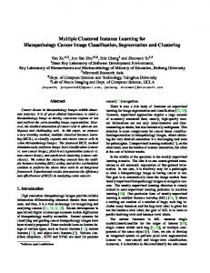
C. Experimental results The comparison and evaluation is divided into two parts. The first experiment evaluates the detection performance of the proposed method, Rieck and AMAL trained on the full training set (121 115 samples), while the second experiment measures degradation of detection performance when only a limited number of data are available for training (5%, 10%, 20% and 100% of training samples). Note that to evaluate AMAL on the complete training set, the meta learner was not allowed to use SVM classifier with RBF kernel due to excessive computational requirements. Note that AMAL’s metalearner has never selected this variant of the SVM classifier in smaller experiments performed in this work, hence removing it most probably does not have any impact on the results. The detection rates and accuracy of classifiers trained on all 121 115 training samples as estimated on testing samples are shown in Table V. The differences between evaluation metrics indicate that the proposed approach outperforms both Rieck and AMAL having the lowest false positive rate and false negative rate. A deeper analysis of the misclassifications produced by the proposed approach revealed that most of the false positives (legitimate binaries classified as malware) were software utilities such as TeamViewer that install themselves into system directories without any user interaction. Since their incidence in the training set was relatively low, the random forest was not able to precisely learn this type of behavior. A second source of errors are false negatives (malware samples classified as benign) where almost 70% are caused by insufficient numbers of training samples (less than 100 samples) from corresponding malware families. Another 11% of false negatives was caused by concept drift as a portion of testing samples exhibited different behaviors than training samples, i.e. created files or registry keys followed different pattern, network communication significantly different URLs, etc. Large gaps between training and testing accuracies for AMAL and Rieck suggest that manually created features and BoW features do not generalize over longer periods of time as well as features created through clustering do. This suggests that clustering removes some randomization of resource names while retaining a large part of information content. Figures 1a and 1b show graphs of FNR and FPR rates for larger sizes of the training set expressed as fraction of the data available for training. For fair comparison the testing set was kept static containing all 110 140 samples collected after November 12, 2016. Both graphs show that the proposed approach is able to achieve lower FNR and FPR using fewer samples. In fact, the proposed approach achieved FNR of 0.052 using just 5% of samples, while Rieck achieved 0.066

using the full training set. Similarly, the proposed approach needed just 20% of samples to achieve the same FPR 0.081 as Rieck on all samples. Figures 1a and 1b also shows that while false negative rates almost do not change with respect to the size of the training set (especially for the proposed approach), the false positive rates decrease dramatically. This suggests that learning behavior of legitimate applications is more difficult than that of malware, which can be caused by the fact that the behavior of malware is more uniform than that of legitimate applications. This corroborates the motivation of this work, that even though malware authors try to randomize, they tend to randomize with same sort of regularity, which leads to uniformity. D. Detection limits The experimental results hint at where are the limits of classifying binaries executed in sandbox. When a binary (or all binaries of some malware family) does not perform any actions changing the data used by the proposed or other methods (files, mutexes, network communication, registry keys) it clearly evades detection. An example of such malware is bitcoin miner that resides only in memory without any additional footprint (no operations with files, no operations with registry keys, no mutexes, very limited network communication). Such malware has to be carefully crafted to avoid any interaction with system resources (statically compiled to carry all libraries in the executable, limited network communication, no mutexes ensuring that only single instance is running on the same machine, no persistency after reboot, etc.). Fortunately, at the time of writing this work, this is not an easy task and the majority of malware authors choose to interact with system resources rather than sacrifice functionality. Another limitation is the fact that a growing number of malware families are equipped with advanced anti-VM and antisandbox features and/or are targeted to specific environments (Stuxnet [13]). Such malware families do not reveal their true purpose during sandboxing or mimic less severe types of malware (adware, PUA6 , etc.). This fact is recognized by the community as the main factor hindering the performance of dynamic analysis as the whole. Addressing this issue is out of the scope of this paper. The last aspect we need to discuss is the false positive rate. The analysis of the results from Section III revealed that a large number of false alarms is caused by applications that install themselves into system directories without user’s interaction and since their number is limited, the classifier was unable to fit this behavior. A solution is of course to improve the training data by including a larger number of such samples and thus achieve lower false positive rate. E. Scalability and computational complexity The last aspect we will discuss is the scalability of the proposed solution and prior art. Since the proposed solution employs clustering to project the input data into a feature space with a lower dimension, a large portion of the training time 6 Potentially

unwanted application.

8

Rieck

Proposed approach

Rieck 0.150

0.100

0.100 FPR

FNR

0.150

Proposed approach

0.050

0.000

0.050

5%

10% 20% Size of training set

100%

(a) False negative rates

0.000

5%

10% 20% Size of training set

100%

(b) False positive rate

Figure 1: Comparison of FNR and FPR for Rieck and proposed method trained on training sets of different sizes (5%, 10%, 20% and 100% of training samples). is spent in the clustering phase. However, the preprocessing of the dataset used in above experiments was much faster (∼ 2h50min) than the highly optimized pre-computation of the full kernel matrix required by Rieck (∼ 7h). This is caused by the fact that the time required by Rieck for preprocessing grows quadratically with the number of training samples in contrast to the proposed solution with linear complexity (up to an additive constant, see Section II-E). Moreover, the proposed solution can be easily distributed since in every iteration the nearest neighbor search depends only on a limited set of current cluster prototypes C ′ . Another benefit of the proposed solution is tied to the representation itself. Since the clustering is performed only on training samples, in order to classify unknown samples we need to store only the cluster prototypes determined during training. For the whole training dataset used in this paper, which contains over 7 million unique resource names projected into ∼ 40 000 features, only 400 000 instances need to be stored. In contrast, the kernelized SVM classifier used by Rieck et al. requires to store all training samples (over 120 000 samples in the data discussed in Section III) with all actions (on average 2000 actions per sample) in order to make prediction on unknown samples. In contrast to both the proposed solution and Rieck, AMAL does not need any preprocessing since the features can be extracted per sample. However, the complexity arises from the design of the training process. Authors in [30] argue that the dynamic selection of both optimal algorithm and its parameters provides optimal results, but this design makes the training process computationally expensive since every training of the meta-learner requires to evaluate all possible combinations of parameters for all its classifiers. Another aspect is the selection of classifiers itself. Authors propose

to use an array of classifiers such as kernelized SVM, linear regression, decision trees, perceptron, etc. However, the complexity of some classifiers (e.g. kernelized SVM) prevents any large-scale training. Moreover, according to the evaluation the AMAL’s detection capabilities are not sufficient for real-world deployment since both FPR and FNR are nearly 20%, which is clearly insufficient. IV. R ELATED WORK Since the analysis of malicious binaries and recommending them for further analysis has important practical applications, there exists rich prior art. Although it is frequently divided into two categories, static and dynamic, the boundaries between them are blurred since techniques such as analysis of the execution graph is used in both categories. A. Static malware analysis Static malware analysis treats a malware binary file as a data file from which it extracts features without executing it. The earliest approaches [27] looked for a manually specified set of specific instructions (tell-tale) used by malware to perform malicious actions but not used by legitimate binaries. Latter works, inspired by text analysis, used n-gram models of binaries and instructions within [26]. Malware authors reacted quickly and began to obfuscate, encrypt, and randomize their binaries, which rendered such basic models [41] useless. Since reversing obfuscation and polymorphic techniques is in theory an NP-hard problem [31], most state of the art [9], [1], [42] moved to a higher-level modeling of sequences of instructions / system calls and estimating their action or effect on the operating system. The rationale behind is that higher-level actions are more difficult to hide.

9

B. Dynamic malware analysis An alternative solution to analyzing obfuscation and encryption is the execution of a binary in a controlled environment and analyzing its interactions with the operating system and system resources. A large portion of the work related to dynamic malware analysis utilize system calls, since in modern operating systems system calls are the only way for applications to interact with the hardware and as such they can reveal malware actions. The simplest methods view a sequence of system calls as a sequence of strings and use histograms of occurrences to create feature vectors for the classifier of choice [17]. The biggest drawback of these naive techniques is low robustness to system call randomization. Similarly to static analysis, this problem can be tackled by assigning actions to groups (clusters) of system calls (syscalls) and using them to characterize the binary [32], [45], [5]. A wide class of methods identifying malware binaries from sequences of syscalls rely on n-grams [24], [34]. Malheur [39] uses normalized histograms of n-grams as feature vectors, which effectively embeds syscall sequences into Euclidean space endowed with L2 norm. In this space the algorithm extracts prototypes Z = {z1 , . . . , zn } using hierarchical clustering. Each prototype captures the behavior of the cluster, which should match corresponding malware family. An interesting feature of Malheur is that if a cluster has less then a certain number of samples, the prototype is not created. The classification of an unknown binary is determined by searching for the nearest prototype within certain range. If the nearest prototype is outside of this range, the sample is not classified. To counter dynamic analysis advanced malware detects the presence of a sandbox and does not execute within it. Since most sandboxes rely on a detectable system call interposition, Das et al. [11] propose to extend hardware with FPGA that would extract system calls from their execution on processor. Syscalls are then grouped by comprehensive yet hand designed rules, and these groups are then fed into multi-layer neural network classifier. The classifier itself is also part of the FPGA, such that the system can simultaneously extract training samples and classify them. AMAL uses its custom sandbox to extract features describing files, network communication and registry features [30] and tunes various classification algorithms. The main difference between AMAL and this work is the construction of features. Whereas AMAL uses numeric features such as counts or sizes of created, modified or deleted files, counts of created, modified or deleted registry keys, counts of unique IP addresses, etc., we assume that individual resources (files, registry keys, mutexes and network communication) have specific role in the operation system, which can be different even though the characteristics exhibited by the file are the same. The approach proposed by Rieck et al. [38] creates a representation of the analyzed binaries directly from the data which is at the first sight similar to the proposed approach, however there are two key differences. The first one is the source of data, because Rieck et al. model actions triggered by

the malware (writing into a file, communication with remote server, reading data from registry keys, starting new thread, etc.), whereas the proposed approach models only affected resources. This enables to deploy the proposed approach in environments without access to low-level actions (VMs without such access, user machines without API hooking). Another difference is in handling the randomization of resource names. Instead of clustering resource names used in this work, Rieck et al. remove parameters of actions, which increases the dimensionality of the model since for every action with n parameters it creates n + 1 features representing the action at different levels of granularity by removing parameters from the end: from full description with all parameters to the most coarse description where only name of the action is used. This leads to a massive increase in the already large number of features.7 Even though the resulting feature space, is sparse the scalability of such an approach is limited. V. C ONCLUSION Dynamic malware analysis is a popular approach to automatically identify malware binaries and analyze them. This paper has proposed a model of malware behavior observed through its interactions with the operating system and network resources (operations with files, mutexes, registry keys, operations with network servers or error messages provided by the operating system). It employs an efficient clustering of resource names to reduce the impact of randomization commonly employed by malware authors to avoid detection and projects malware samples into a low-dimensional space suitable for classifiers such as random forest. The proposed solution was extensively compared to related state of the art on a large corpus of binaries where it demonstrated significant increase in precision of malware detection. Moreover, we believe that the availability of solutions relying on widely different types of features increases the overall reliability of malware detection techniques, because malware authors have to evade more detectors to stay undetected. R EFERENCES [1] Mansour Ahmadi, Dmitry Ulyanov, Stanislav Semenov, Mikhail Trofimov, and Giorgio Giacinto. Novel Feature Extraction, Selection and Fusion for Effective Malware Family Classification. In Proceedings of the Sixth ACM Conference on Data and Application Security and Privacy, pages 183–194, nov 2016. [2] Jaume Amores. Multiple instance classification: Review, taxonomy and comparative study. Artificial Intelligence, 201:81–105, aug 2013. [3] AV-Test. AV-Test Malware Statistics. Technical report, 2016. [4] AV-Test. Consumer Full Product Testing November/December 2016. Technical report, AV-TEST GmbH, 2016. [5] Ulrich Bayer, PM Paolo Milani Comparetti, Clemens Hlauschek, Christopher Kruegel, and Engin Kirda. Scalable, Behavior-Based Malware Clustering. In Proceedings of the 16th Annual Network and Distributed System Security Symposium (NDSS 2009), 2009. [6] Christopher M Bishop. Pattern recognition and machine learning, volume 4. Springer, 2011. [7] Vincent D. Blondel, Jean-Loup Guillaume, Renaud Lambiotte, and Etienne Lefebvre. Fast unfolding of communities in large networks. Journal of Statistical Mechanics: Theory and Experiment, 2008(10):P10008, mar 2008. [8] Leo Breiman. Random Forests. Machine Learning, 45(1):5–32, 2001. 7 According to the experiments, the number of features generated for about 6000 samples reaches over 20 million.

10

[9] Mihai Christodorescu and Somesh Jha. Static Analysis of Executables to Detect Malicious Patterns. Technical report, Computer Sciences Department University of Wisconsin, Madison, 2006. [10] Corinna Cortes, Mehryar Mohri, and Afshin Rostamizadeh. Algorithms for Learning Kernels Based on Centered Alignment. The Journal of Machine Learning, mar 2012. [11] Sanjeev Das, Yang Liu, Wei Zhang, and Mahintham Chandramohan. Semantics-Based Online Malware Detection: Towards Efficient RealTime Protection Against Malware. IEEE Transactions on Information Forensics and Security, 11(2):289–302, feb 2016. [12] Artem Dinaburg, Paul Royal, Monirul Sharif, and Wenke Lee. Ether: Malware Analysis via Hardware Virtualization Extensions. In Proceedings of the 15th ACM conference on Computer and communications security - CCS ’08, page 51, New York, New York, USA, 2008. ACM Press. [13] Nicolas Falliere, Liam O Murchu, and Eric Chien. W32.Stuxnet Dossier analysis report. Technical report, 2011. [14] Tom Fawcett. An introduction to ROC analysis. Pattern Recognition Letters, 27(8):861–874, jun 2006. [15] Santo Fortunato. Community detection in graphs. Physics Reports, 486(3-5):75–174, feb 2010. [16] David Reguera Garcia. AntiCuckoo. [17] Steven Strandlund Hansen, Thor Mark Tampus Larsen, Matija Stevanovic, and Jens Myrup Pedersen. An approach for detection and family classification of malware based on behavioral analysis. In 2016 International Conference on Computing, Networking and Communications (ICNC), pages 1–5. IEEE, feb 2016. [18] CISCO Systems Inc. AMP ThreatGrid. [19] Google Inc. VirusTotal.com. [20] Jiyong Jang, David Brumley, and Shobha Venkataraman. BitShred : Fast , Scalable Malware Triage. Technical report, 2010. [21] Jan Jusko, Martin Rehák, Jan Stiborek, Jan Kohout, and Tomáš Pevný. Using Behavioral Similarity for Botnet Command and Control Discovery. IEEE Intelligent Systems, 2016. [22] Gaurav S Kc, Angelos D Keromytis, and Vassilis Prevelakis. Countering code-injection attacks with instruction-set randomization. In Proceedings of the 10th ACM conference on Computer and communication security - CCS ’03, page 272, New York, New York, USA, 2003. ACM Press. [23] Jan Kohout and Tomas Pevny. Automatic discovery of web servers hosting similar applications. In Proceedings of the 2015 IFIP/IEEE International Symposium on Integrated Network Management, IM 2015, pages 1310–1315, 2015. [24] Andrea Lanzi, Davide Balzarotti, Christopher Kruegel, Mihai Christodorescu, and Engin Kirda. AccessMiner: Using SystemCentric Models for Malware Protection. In Proceedings of the 17th ACM Conference on Computer and Communications Security – CCS’10, pages 399–412, 2010. [25] Vladimir I. Levenshtein. Binary codes capable of correcting deletions, insertions, and reversals. Soviet Physics Doklady, 10(8):707–710, 1966. [26] Wei Jen Li, Ke Wang, Salvatore J. Stolfo, and Benjamin Herzog. Fileprints: Identifying file types by n-gram analysis. Proceedings from the 6th Annual IEEE System, Man and Cybernetics Information Assurance Workshop, SMC 2005, 2005(July 2005):64–71, 2005. [27] Raymond W. Lo, Karl N Levitt, and Ronald A Olsson. MCF: a malicious code filter. Computers & Security, 14(6):541–566, jan 1995. [28] Huma Lodhi, Craig Saunders, John Shawe-Taylor, Nello Cristianini, and Chris Watkins. Text Classification using String Kernels. Journal of Machine Learning Research, 2:419–444, 2002. [29] Weiqin Ma, Pu Duan, Sanmin Liu, Guofei Gu, and Jyh Charn Liu. Shadow attacks: Automatically evading system-call-behavior based malware detection. Journal in Computer Virology, 8(1-2):1–13, 2012. [30] Aziz Mohaisen, Omar Alrawi, and Manar Mohaisen. AMAL: Highfidelity, behavior-based automated malware analysis and classification. Computers & Security, 52:251–266, jul 2015. [31] Andreas Moser, Christopher Kruegel, and Engin Kirda. Limits of static analysis for malware detection. In Proceedings - Annual Computer Security Applications Conference, ACSAC, pages 421–430. IEEE, dec 2007. [32] Smita Naval, Vijay Laxmi, Muttukrishnan Rajarajan, Manoj Singh Gaur, and Mauro Conti. Employing Program Semantics for Malware Detection. IEEE Transactions on Information Forensics and Security, 10(12):2591–2604, dec 2015. [33] Gonzalo Navarro. A guided tour to approximate string matching. ACM Computing Surveys, 33(1):31–88, mar 2001.

[34] Philip O’Kane, Sakir Sezer, Kieran McLaughlin, and Eul Gyu Im. SVM Training Phase Reduction Using Dataset Feature Filtering for Malware Detection. IEEE Transactions on Information Forensics and Security, 8(3):500–509, mar 2013. [35] Digit Oktavianto and Iqbal Muhardianto. Cuckoo Malware Analysis. Packt Publishing, 2013. [36] Fabian Pedregosa, Gaël Varoquaux, Alexandre Gramfort, Vincent Michel, Bertrand Thirion, Olivier Grisel, Mathieu Blondel, Peter Prettenhofer, Ron Weiss, Vincent Dubourg, Jake Vanderplas, Alexandre Passos, David Cournapeau, Matthieu Brucher, Matthieu Perrot, and Édouard Duchesnay. Scikit-learn: Machine Learning in Python. Journal of Machine Learning Research, 12(Oct):2825–2830, 2011. [37] William M Rand. Objective Criteria for the Evaluation of Clustering Methods Objective Criteria for the Evaluation of Clustering Methods. Journal of the American Statistical Association, 66(336):846–850, 1971. [38] Konrad Rieck, Thorsten Holz, Carsten Willems, Patrick Dussel, and Pavel Laskov. Learning and classification of malware behavior. Detection of Intrusions and . . . , 2008. [39] Konrad Rieck, Philipp Trinius, Carsten Willems, and Thorsten Holz. Automatic analysis of malware behavior using machine learning. Journal of Computer Security, 19(4):639–668, jun 2011. [40] Marcos Sebastián, Richard Rivera, Platon Kotzias, and Juan Caballero. AVclass: A Tool for Massive Malware Labeling. In Research in Attacks, Intrusions, and Defenses: 19th International Symposium, RAID 2016, Paris, France, September 19-21, 2016, Proceedings, pages 230–253, 2016. [41] Monirul Sharif, Andrea Lanzi, Jonathon Giffin, and Wenke Lee. Impeding Malware Analysis Using Conditional Code Obfuscation. Informatica, 2008. [42] Monirul Sharif, Vinod Yegneswaran, Hassen Saidi, Phillip Porras, and Wenke Lee. Eureka: A framework for enabling static malware analysis. In Lecture Notes in Computer Science (including subseries Lecture Notes in Artificial Intelligence and Lecture Notes in Bioinformatics), volume 5283 LNCS, pages 481–500, 2008. [43] Symantec Security Response. Sality: Story of a Peer- to-Peer Viral Network. Technical report, Symantec, Inc., 2011. [44] Carsten Willems, Thorsten Holz, and Felix Freiling. Toward Automated Dynamic Malware Analysis Using CWSandbox. IEEE Security and Privacy Magazine, 5(2):32–39, mar 2007. [45] Tobias Wüchner, Martín Ochoa, and Alexander Pretschner. Malware detection with quantitative data flow graphs. Proceedings of the 9th ACM symposium on Information, computer and communications security - ASIA CCS ’14, pages 271–282, feb 2014. [46] Tian Zhang, Raghu Ramakrishnan, and Miron Livny. BIRCH: A New Data Clustering Algorithm and Its Applications. Data Mining and Knowledge Discovery, 1(2):141–182, 1997. [47] Arthur Zimek, Matthew Gaudet, Ricardo J.G.B. G B Campello, and Jörg Sander. Subsampling for efficient and effective unsupervised outlier detection ensembles. In Proceedings of the 19th ACM SIGKDD international conference on Knowledge discovery and data mining KDD ’13, page 428, 2013.

A PPENDIX A. Frobenius product and Frobenius norm For two matrices A ∈ Rn×m and B ∈ Rn×m we define Frobenius product h·, ·iF and Frobenius norm k·kF as follows hA, BiF =

m n X X

Aij · Bij

i=1 j=1

v uX m q u n X A2ij kAkF = hA, AiF = t i=1 j=1