Multiple Instance Learning for Soft Bags via Top Instances

Multiple Instance Learning for Soft Bags via Top Instances Weixin Li Nuno Vasconcelos University of California, San Diego La Jolla, CA 92093, United States {wel017, nvasconcelos}@ucsd.edu Abstract A generalized formulation of the multiple instance learning problem is considered. Under this formulation, both positive and negative bags are soft, in the sense that negative bags can also contain positive instances. This reflects a problem setting commonly found in practical applications, where labeling noise appears on both positive and negative training samples. A novel bag-level representation is introduced, using instances that are most likely to be positive (denoted top instances), and its ability to separate soft bags, depending on their relative composition in terms of positive and negative instances, is studied. This study inspires a new large-margin algorithm for soft-bag classification, based on a latent support vector machine that efficiently explores the combinatorial space of bag compositions. Empirical evaluation on three datasets is shown to confirm the main findings of the theoretical analysis and the effectiveness of the proposed soft-bag classifier.

negative bags positive bags

X

negative instance positive instance (positive bag) (positive bag) (negative bag) (negative bag)

separating plane

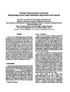
Figure 1. Noisy weak annotation of “flower” in Corel5k, where negative bags are far more than positive bags in training data. Best viewed in color (same for the rest).

beling of negatives is as noisy as that of positives. Figure 1 illustrates the problem for the popular Corel5k dataset [4]. Image patches are considered instances of visual concepts and the goal is to classify images, which are bags of such patches, with concept labels. The figure shows examples of positive and negative bags for the concept “flower”. Note that many of the negative images include regions of flowers. This labeling noise is common in weakly supervised learning, where human annotators are asked to label data with a few keywords. The absence of the “flower” label does not mean that there are no flowers in the image, just that the labeler did not think of “flower” as one of its predominant concepts. In result, negative bags frequently contain positive instances. This nullifies the core MIL assumption of clean negative bags. To address this common issue, we consider a more general definition of MIL, which softens its constraint on negative bags. Under this formulation, both positive and negative bags are soft (i.e., they can contain both positive and negative instances, differing only in their composition with regards to the two instance types). This is unlike the hard bags of conventional MIL (where presence/absence of posi-

1. Introduction Multiple instance learning (MIL) [9] is a family of learning algorithms suitable for problems involving substantial amounts of labeling noise. Examples, denoted as instances in MIL, are grouped into bags, and a label is attached to each bag. A bag that contains at least one positive example is considered a positive bag, otherwise it is negative. A classifier is finally designed to classify bags, rather than individual examples. Over the past twenty years, many MIL algorithms have been developed and successfully applied to different tasks where label noise is prevalent, e.g., image categorization [16, 6, 5], object detection [22, 10], retrieval [16, 29, 4], etc. While a substantial step towards the development of systems that can learn from very weakly labeled data, the current formulation of MIL fails to account for a very characteristic property of this type of data: negative bags can also have very noisy instance composition. In fact, for some of the most popular applications of MIL, e.g., semantic annotation of images or video, the la1

tive instances makes a bag positive/negative). This is shown to generalize both supervised learning and conventional MIL, but is applicable to a much broader range of problems. While a similar setting has been suggested before by [25], its solution relies on a heuristic two-phase procedure that does not fully exploit the properties of the problem. In this work, our technical contribution goes far beyond [25]. We propose a new bag representation for separating soft positive and negative bags. This relies on the bag instances that are most likely to be positive (denoted top instances) to construct a feature that remains discriminant in the softbag setting. A detailed study of the separability of this feature, depending on the relative compositions of positive and negative bags is then presented, establishing connections to several previous works. Several theoretical results on soft bag separability are derived, motivating a new large-margin solution of the soft-bag MIL problem based on a latent support vector machine (SVM). This effectively and efficiently exploits a combinatorial number of possible bag representations to achieve a provably optimal solution. Empirical evaluation on three datasets, including both conventional and soft-bag MIL, confirms the main theoretical findings on soft-bag separability, and demonstrates the effectiveness of the approach.

2. Related Works MIL was introduced by [9] to address the problem of drug prediction, where a positive bag is exclusively identified by one significant positive instance. Various solutions and applications have since been proposed, based on both generative [16, 4] and discriminant [1, 11, 25, 6, 5, 3, 31, 15, 30, 8, 12] formulations of the problem. Early works posed MIL as the identification of the single positive instance in a positive bag, learning a prediction rule that separates it from negative instances [9, 16, 29, 1]. Various later works showed that robust MIL solutions require understanding of the instance distributions of bags. [11] designed a holistic bag representation by merging all instances into a single feature vector. [31] investigated the relation between MIL and semi-supervised learning. [3] showed that when positive instances are sparse in positive bags, it is desirable to extract them before making the final prediction. [30] modeled relations among instances in a bag via a graph, using graph kernels to encode bag-level similarity for discrimination. [8] proposed a conditional random field that combines unary instance classifiers and pairwise measures of bag dissimilarity. [12] studied the structure of positive bags and proposed a projection operator to learn robust MIL classifiers. All these approaches follow the original MIL formulation, assuming that all instances of negative bags are negative examples. A few works have tried to relax this assumption, acknowledging the labeling noise in negative bags. [25] com-

plemented MIL with three such assumptions, which justify an alternative two-layer quantize-then-classify (TLC) MIL algorithm. [24] formulated MIL as an adaptive procedure to determine instance-to-bag soft assignments, using a bag-level feature based on the p-th power of instance aggregate posterior probabilities, generalizing the hard assignment of TLC. While, as discussed in Section 3 and Section 4.2, some of these formulations have commonalities with the proposed soft-bag MIL, they mostly rely on positive instances for bag separation. This fails to consider the negative instances of negative bags, which are shown to further improve the separability of soft bags in this work. It should also be noted that the soft-bag image annotation problem of Figure 1 is related to the semi-supervised multiple-label image tagging problem of, e.g., [19]. However, in this setting 1) a bag is represented by a single instance, 2) this instance is associated with multiple labels as a whole, and 3) only a portion of the positive bags for a given concept are annotated. This is different from the soft-bag setting that we investigate, where all bags are annotated, but not with the proverbial “1,000 words” that a picture is worth. Instead, reflecting the well known “popout” effect of dominant attributes in human perception, it is the predominance rather than the presence of a visual concept in an image that makes a human annotator label the image with that concept [17, 21].

3. Definitions A soft bag B is a set of instances, or examples, x ∈ X ⊆

RD . Instances are sampled independently from two distri-

− butions p+ X (x) (denoted positive source) and pX (x) (denoted negative source). The positive source is the distribution of the target concept (e.g., image patches of “flower”), the negative source the distribution of background clutter (e.g., image patches of everything else). B Definition 1. A soft bag B = {xi }N i=1 is a set of NB instances, where NB > N and N ∈ Z++ is a lower bound on bag size, sampled as follows

• sample NB+ from a probability mass function p(NB+ = i) with 0 6 i 6 NB ; N+

B • sample NB+ i.i.d. instances {xi }i=1 from the positive + source pX (x); B • sample NB− = NB − NB+ i.i.d. instances {xi }N i=N + +1

from the negative source p− X (x).

B

The bag label y ∈ Y = {−1, +1} is determined as follows. Definition 2. Let 0 < µ 6 N be a lower bound on the number of positive examples per positive bag. A soft bag B is µ-positive (label +1) if NB+ > µ and µ-negative (label −1) otherwise.

It follows that, while a µ-negative soft bag can contain positive instances, the number of these has to be less than that of a µ-positive soft bag. The goal is to predict if a query bag Bq is µ-positive or µ-negative, i.e., to learn a prediction rule f : X NB 7→ Y, from a training dataset D = {(Bi , yi )}. Note that this definition generalizes the conventional MIL and supervised learning problems. Conventional supervised learning corresponds to NB = µ = 1, where a bag contains either a positive or negative instance. Conventional MIL corresponds to µ = 1, where a positive bag contains at least one instance from p+ X (x) and all instances in a negative bag are from p− (x). However, the classification of soft bags X is more complex than that of conventional MIL bags, since a µ-negative soft bag can contain positive instances when µ > 1. For example, since both positive and negative bags are expected to contain both positive and negative examples, the conventional definition of class separability makes little sense for soft-bag MIL. What matters is the separability of the source distributions. This is the motivation for the following definition. Definition 3. The soft bag classification problem is denoted − separable if the regions of support of p+ X (x) and pX (x) are linearly separable, i.e., if there exists a linear prediction − rule fX : X 7→ R such that ∀ x+ ∈ supp(p+ ∈ X ), x − supp(pX ), fX (x+ ) > 0 > fX (x− ). (1) fX is denoted a separator of the soft bag problem. Figure 2 illustrates a separable soft bag classification problem with N = 8. Denoting the positive (negative) bag by Bp (Bn ), the figure depicts a scenario where 1 Nn+ = 1, and Np+ = 4. As usual, while we base the definition on the linear separability of the instance space X , all results apply if linear separability holds in a reproducing kernel Hilbert space (RKHS), after application of the kernel trick. It should be noted that both the definitions above and the analysis that follows can be extended to a slightly different formulation of the problem, where positive and negative soft bags differ in the proportion of their positive instances (as opposed to the absolute number). This extension is discussed in the supplementary material.

4. Separability of Soft Bags via Top Instances In this section, we study the separability of positive and negative soft bags.

4.1. Representation of Soft Bags by Top Instances Consider a separable soft bag MIL problem with separator f . Since positive bags have more positive instances than + 1 For simplicity, we use the shorthand notations N for N n Bn and Nn + + for NB (similar for N , N ) in the rest of the paper. p p n

negative instance (positive bag) (negative bag)

ΦB,2

positive instance (positive bag) (negative bag)

(positive bag) (negative bag)

fX (x)

supp(p− X)

X

ξ

δ b− u

supp(p+ X)

b+ l

0

b+ u

s

Figure 2. MIL for soft bags. The two contours delimit the support sets of the two sources. Positive and negative instances are identified by symbol shape, their bag ownerships by color (see insets). The top 2 instances are used to represent each of the two bags (one positive and one negative). These are the instances connected by a dotted line. For the other variables please see the text.

negative bags, it is natural to represent a bag B by a compound feature Φf,k of its k (1 6 k 6 NB ) “most positive” instances 1X Φf,k (B) = xi (2) xi ∈Ω∗ k f,k (B) with Ω∗f,k (B) = argmax

Ω⊆B,|Ω|=k

X xi ∈Ω

f (xi ).

In what follows, we refer to the instances in Ω∗f,k (B) as the top instances of B according to separator f (see Figure 2). Under the top instance representation, the application of the linear separator f (x) to a bag B produces a bag score   X X 1 1 sf,k (B) = f xi = f (xi ). k k ∗ ∗ xi ∈Ωf,k (B)

xi ∈Ωf,k (B)

(3) Φf,k (B) generalizes features of various MIL methods. When k = 1, it reduces to the feature of the MI-SVM [1], which represents a bag by its most positive instance with respect to f . On the other hand, when k = NB+ for positive bags, Φf,k (B) is the feature used by the sparse-bag SVM [3] and TLC [25], which represent a positive bag by its positive instances. Finally, when k = NB , Φf,k (B) is the feature of the 1-norm normalized set kernel (NSK) of [11], which represents each bag by the mean of all its instances. We will later see that these choices are only optimal for special classes of soft bags. For now, we study the separability of soft bags under the feature representation of (2).

4.2. Soft Bag Separability Given the bag scores of (3), the separability score, under separator f , of a µ-positive soft bag Bp and a µ-negative

(4)

The bags are said to be Φf,k -separable if ∆sf,k (Bp , Bn ) > 0. The following theorem characterizes how the expected value of ∆sf,k (Bp , Bn ) depends on k. Theorem 1 (Expected separability). Consider a separable MIL problem of separator f and let Bp be a µ-positive and Bn a µ-negative soft bag with Np+ and Nn+ positive instances, respectively, where 0 6 Nn+ < µ 6 Np+ 6 N . Let ∆Sf,k be the random variable from which the separability scores ∆sf,k of (4) are drawn. 1. If 1 6 k 6 Nn+ − 1, then

N+p=10, N+p=10,

1.5 E[ S(k)]

∆sf,k (Bp , Bn ) = sf,k (Bp ) − sf,k (Bn ).

N+p=15, N+n=10 N+n=2 N+n=0

0.4

0.3

1

0.2

0.5

0.1

0 0

5

10

15

20 k

25

30

35

40

Var[ S(k)]

2

soft bag Bn is

0

Figure 3. Illustration of E [∆Sf,k (Bp , Bn )] (solid curves) and Var (∆Sf,k (Bp , Bn )) (dotted curves). S + ∼ U (1, 2), S − ∼ U (−3, −1) for red curve; S + ∼ U (0, 1), S − ∼ U (−1, 0) for blue; and S + ∼ U (0.1, 0.2), S − ∼ U (−5, −0.5) for black.

0 6 E [∆Sf,k (Bp , Bn )] 6 E [∆Sf,k+1 (Bp , Bn )] . (5) 2. If Nn+ < k 6 Np+ , then h i 0 6 E ∆Sf,Nn+ (Bp , Bn ) 6 E [∆Sf,k (Bp , Bn )] . (6) 3. For any finite Np+ , limN →∞ E [∆Sf,N (Bp , Bn )] = 0.

(7)

Proof: See the supplemental material (same for others). The first statement of the theorem shows that, while expected Φf,k -separability is guaranteed for all k 6 Nn+ , the expected value of ∆Sf,k (Bp , Bn ) is non-decreasing with k. It can also be shown that an upper bound of the variance of the separability score decreases with k (see supplemental material, same for the rest). It follows that there is no advantage in using k smaller than Nn+ − 1 in (2). The second statement then shows that using more than the Nn+ top instances (but no more than Np+ ) leads to an even larger expected separability score. This is intuitive since, in this regime, Φf,k (Bp ) only includes scores of positive instances xi (for which f (xi ) is positive) while Φf,k (Bn ) includes scores from k − Nn+ negative instances (for which f (xi ) is negative). Finally, the third statement shows that there is no advantage in using a number of top instances much larger than Np+ . For large bags (N → ∞) with small number of positive instances, using all instances (k → ∞) leads to zero expected separability. This is again intuitive since, in this regime, bag scores are dominated by negative instances and there is little hope of bag discrimination. Overall, the theorem shows that, whenever µ-negative bags have more than one positive example (Nn+ > 0), there exist values of k (Nn+ < k 6 Np+ ) for which the feature of (2) is more discriminant than that of MISVM (k = 1). Note that this may also hold under the standard MIL assumptions, i.e., µ = 1 (Nn+ = 0). This behavior is illustrated by Figure 3, which

presents curves of E [∆Sf,k (Bp , Bn )] (solid lines) and Var (∆Sf,k (Bp , Bn )) (dotted lines) for three separable softbag MIL problems of uniform bag score distributions pS . In the black example (Np+ = 10, Nn+ = 0), which falls within the MI setting of µ = 1, the expected separability of k = 1, as in the MI-SVM, is significantly smaller than the maximum value (k = 10). On the other hand, the theorem shows that the NSK setting (k = NB ) of using all instances in (2) compromises bag separability, at least when bags are large and positive instances are sparse (this resembles the observation of [3]). This is visible in all examples of Figure 3, where large k lead to low separability in all examples. Finally, the largest expected separability is usually obtained for values of k that lie within these two settings, namely Nn+ < k 6 Np+ . Note, however, that there is no guarantee that this happens for k = Np+ , as advocated by sparse-bag SVM [3] and TLC [25]. In Figure 3, this has the largest separability for the red example (Np+ = 15, Nn+ = 10), but not for the blue one (Np+ = 10, Nn+ = 2). One particularly interesting choice of k is k = µ. In this case, separability holds not only in expected value but for any sample, if certain conditions holds ( for a visualization of the bounds in the theorem see Figure 2). Theorem 2 (Absolute separability). Consider an MIL problem linearly separable by prediction rule fX with µ-positive soft bags Bp and µ-negative soft bags Bn . Let b+ u = + sup{fX (x)|x ∈ supp(p+ )}, b = inf{f (x)|x ∈ X X l − − supp(p+ )}, and b = sup{f (x)|x ∈ supp(p )}. If the X u X X number of positive instances in any µ-negative soft bag Bn satisfies  +    bl − b− 1 u + Nn 6 τ = µ + = µ , (8) 1 + ξ/δ bu − b− u

− where δ = b+ l − bu is the margin of the classification prob+ lem and ξ = bu − b+ l a measure of compactness of the

positive source, then, under the representation of (2), any pair Bp , Bn is separable by fX (x) at k = µ, i.e., fX (ΦfX ,µ (Bp )) > fX (ΦfX ,µ (Bn )).

(9)

It is worth making two notes. First, condition (8) does not require that the total number of positive instances across all negative bags be upper-bounded. In fact, this number could be arbitrarily large, as long as the condition holds for each single negative bag. The bound implies that the allowable number of positive instances in a µ-negative bag increases when the margin δ is larger or the positive source more compact (smaller ξ). Second, (8) implies that the number of negative instances in any negative bag has to exceed NB − τ . While intuitive, since the negative examples are what distinguishes the top instances of the two bags “pulling down” the score sf,k (Bn ) of negative bags and increasing the separability measure of (4) - this fact has received little attention in the MIL literature. In what follows, we will exploit it for improved performance.

4.3. Consistency with Supervised Learning The separability of a soft-bag representation ΦfX ,k (·) should increase with additional labeling of the instances in each bag. In the limit of fully labeled instances, i.e., an oracle that assigns labels to all instances, soft bag separability should be as high as the separability δ of the source distributions. When this happens, the representation ΦfX ,k (·) is said to be consistent with supervised learning. So far, we have assumed that all instances are equally weighted in the bag representation of (2). Since Ω∗f,k (B) contains more negative instances for a µ-negative than for a µ-positive bag, the assignment of larger weights to negative instances would increase the prediction score of (4). Hence, separability would increase if heavier weights were assigned to negative instances. Let di = g(xi ) be a weighting function. Given a bag B, the representation of (2) can be generalized to a weighted compound feature ΦfX ,k (B) = Φ(X, h∗ ) =

Xh∗ , dT h∗

(10)

with

Theorem 3 (Consistency with supervised learning). Let − − γ = sup{g(x+ )/g(x− )|x+ ∈ supp(p+ X ), x ∈ supp(pX )}. + + If Nn < k 6 Np , then, under the bag representation of (10), lim inf ∆Sf,k (Bp , Bn ) > δ, (11) γ→0

where δ is the margin as defined in Theorem 2. Note that γ → 0 if g(x+ )  g(x− ) for all pairs (x , x− ). Since, when δ > 0, this holds if g(xi ) is the indicator function of negative instances, the condition of the theorem holds whenever an oracle is available to label all instances. Hence, if the source distributions are separable, the representation of (10) is consistent with supervised learning. +

4.4. Weighting Functions The discussion above suggests that improved MIL performance may be possible by replacing the representation of (2) with that of (10). It remains to determine an effective weight function g(x). While an oracle is not available in practice, it may suffice to use an approximation of the indicator of negative examples. In this work, we consider + a combination of the consistent estimator p˜+ X (x) of pX (x) from [4] and the logistic transformation  −1 g(x) = 1 + exp(α log p˜+ , (12) X (x) + β) where α ∈ R++ and β are scaling and offset parameters determined by cross-validation. Note that many other choices of weight functions would be possible. The determination of the optimal weighing function is a topic that we leave for future work.

5. Classification with Soft Bags For now, we consider the design of a soft bag classifier with the feature of (10).

5.1. Prediction Rule and Inference Given a bag B, the prediction rule that quantifies the confidence of B being positive with k top instances is X fw (XB ) = maxh∈H wT Φ(XB , h), hi = k, (13) i

h∗ = argmax fX h∈H



Xh dT h

D

 , s.t.

X i

hi = k,

D×N

B where X = [x1 , x2 , · · · , xNB ] ∈ R is a matrix whose columns are the instances of B, d = NB [d1 , · · · , dNB ]T ∈ R++ the vector of weights, and h∗ ∈ P NB H = {0, 1} \ {0} ( i hi = k 6 NB ) an indicator function for the top instances of bag B. Note that when di = 1, ∀i, (10) reduces to (2). The following theorem shows that (10) is consistent with supervised learning.

where w ∈ R is the vector of predictor coefficients, D Φ(XB , h) ∈ R the feature vector of (10), h a vector of latent variables, H the hypothesis space {0, 1}NB \ {0}. The prediction of (13) requires the solution of X w T XB h , s.t. hi = k. (14) T i h∈H d h Since the indicator variable h is discrete, this is a integer linear-fractional programming (ILFP). Note that, given d ∈ B RN ++ , it can be solved efficiently, via the solution of a linear programming by the following result. (ILFP) :

max

1

1

1

1

0.8

0.8

0.8

0.8

0.6

0.6

0.6

0.6

0.4

0.4

0.4

0.4 1.00−0.00 1.00−0.20 1.00−0.40 1.00−0.60 1.00−0.80

0.20−0.00 0.40−0.00

0.2

0.2

0.40−0.20

0 0

4

8

12

16

20

0 0

0.60−0.00 0.60−0.20 0.60−0.40

4

8

12

k

16

20

k

0.80−0.00 0.80−0.20 0.80−0.40 0.80−0.60

0.2 0 0

4

8

12

16

k

20

0.2 0 0

4

8

12

16

20

k

Figure 4. Classification accuracy on 15 synthetic datasets that differ in the percentage of positive instances per bag. The numbers shown in the legend are the proportions of positive instances in a positive (ηp+ ) and negative (ηn+ ) bag, respectively. Solid curves correspond to unweighted, dashed curves to weighted results (same for other figures).

Theorem 4 (Exact linear relaxation). If d  0 (i.e., ∀i, di is strictly positive), the optimal value of (14) is identical to that of the relaxed problem X w T XB h (LFP) : max , s.t. hi = k, (15) i h∈BNB dT h NB

where B NB = [0, 1]NB is a unit box in R

.

Since (15) is a linear-fractional programming (LFP), it can be reduced to a linear programming (LP) of NB + 1 variables and NB + 2 constraints [2]. It follows that exact inference can be performed efficiently for the max-margin latent variable classifier of (13) with combinatorial composition space.

5.2. Learning The learning problem is to determine the parameter vecT tor w, given a training set D = {Bi , yi }N i=1 . This is a latentSVM learning problem [10] XNT
1 min ||w||2 + C max 0, 1 − yi fw (XBi ) . w 2 i=1 (16) In this work, we adopt the concave-convex procedure (CCCP) of [27] as the solver. This consists of rewriting the objective of (16) as the difference of two convex functions  min w

X
1 ||w||2 + C max 0, 1 + fw (XBi ) + 2 i∈Dn   X  (17) X
C max fw (XBi ), 1 − C fw (XBi ) , i∈Dp

i∈Dp

where Dp and Dn are the positive and negative training sets, respectively. CCCP then alternates between two steps until convergence . The first computes a tight convex upper bound of the second (concave) term of (17), by estimating the configuration of hidden variables that best explains the positive training data using the current model. The second minimizes this upper bound, by solving a structural SVM [20] problem, which is convex, via the proximal bundle method [14]. The initial w is learnt with a SVM by N setting h = 1 ∈ R B , which empirically produces a reasonably good result to start the learning procedure.

6. Experiments In this section, we report on an empirical evaluation of soft-bag MIL.

6.1. Synthetic Data To provide some intuition on the behavior of the proposed soft-bag SVM, we conducted an experiment with 15 synthetic datasets of different instance distributions for positive and negative bags. In all cases the instance space is 2 X = R , the sources Gaussian, with p+ X (x) = N (x; 2, 1) − and pX (x) = N (x; −4, 10), and every bag contains NB = 20 instances. The 15 datasets differ in the percentage of positive instances in either positive or negative bags (denoted ηp+ and ηn+ , respectively). Each dataset contains 200 positive and 1000 negatives bags, which are split equally between a training and a test set. A two-component Gaussian mixture model (GMM) was used to learn the weighting function of (12). Figure 4 shows the classification accuracy for each dataset, for both uniform and GMM-based weighting, as a function of the number k of top instances. Overall, these results confirm the predictions of our analysis on the separability of soft bags in Section 4.2. For example, in almost all datasets, classification accuracy increases with k, when k is smaller than the number of positive instances per negative bag (k = 1 to k = 20 × ηn+ ). Around this critical point (k = Nn+ ), there is typically a surge in accuracy (note the behavior around k = 20 × ηn+ in curves “0.80-0.20”, “0.80-0.60”, “1.00-0.80”, etc), and classification performance is consistently better for 20 × ηn+ < k 6 20 × ηp+ than for k 6 20 × ηn+ . This reflects the benefit of forcing negative bags to include negative instances, increasing bag separability. Furthermore, while accuracy typically increases with k for 20 × ηn+ < k 6 20 × ηp+ , there are many cases where k = 20 × ηp+ does not guarantee best performance. In fact, most of the accuracy maxima are located in k ∈ (20 × ηp+ , 20). For the sources used in this experiment, it is favorable to include some negative instances even in positive bags. This may be due to the fact that the Gaussian sources are not separable, which could introduce a lag in the optimal value of k. Finally, the use of the GMM-based weighting function

Table 1. Classification accuracy (%) on benchmark MIL datasets. method

Musk1

Musk2

Elep.

Fox

Tiger

EM-DD [28] MI-SVM [1] NSK [11] TLC [25] MI/LR [18] sbMIL [3] PPMM [24] miGraph [30] PC-SVM [12] CRF-MIL [8] Con. Rel.-WSC [13]

84.8 77.9 88.0 88.7 85.4 89.8 95.6 88.9 90.6 88.0 87.7

84.9 84.3 89.3 83.1 87.1 87.3 81.2 90.3 91.3 85.3 N/A

78.3 81.4 84.3 80.5 89.3 88.0 82.4 86.8 89.8 85.0 86.7

56.1 59.4 60.3 62.4 63.1 69.0 60.3 61.6 65.7 67.5 62.5

72.1 84.0 84.2 82.2 86.2 82.1 80.2 86.0 83.8 83.0 78.0

soft-bag SVM w/o weight soft-bag SVM weighted (average # instances per bag)

90.3 89.6 (5.2)

88.5 90.2 (64.7)

89.0 89.5 (7.0)

69.0 67.7 (6.6)

86.5 86.0 (6.1)

usually improves performance, with improvements as large as 10%.

6.2. Benchmark MIL Datasets The second set of experiments was conducted on two benchmark MIL datasets: Musk [9] and Corel-Animal [1]. Here, we followed the standard evaluation protocol from the literature and reported results via 10-fold cross-validation. The performance of the proposed soft-bag SVM is shown as a function of k in Figure 5. Note that, in three of the datasets, best performance is obtained with two top instances (k = 2). This reflects the fact that the majority of bags in these datasets only contain one or (possibly) two positive instances and there is usually no positive instance in negative bags. This is not surprising, since these datasets are benchmarks for conventional MIL, where this setting is assumed. Table 1 compares various methods, based on per-fold average classification accuracy (the top two results are bolded for each dataset). The optimal k of our method was determined by cross validation on the training set (same for Table 2). These results show that, even in the conventional MIL scenario, the soft-bag SVM is a top performer. It achieves one of two best results on three animal datasets and results competitive with the best in the remaining two (“Musk”). In fact, the soft-bag SVM with uniform weights has the best performance on two datasets. The only other method with two “wins” is PC-SVM. The last row of the table details the average number of instances per bag for each dataset. The superior performance of the unweighted soft-bag SVM, is explained by the fact that most datasets have very small bags, e.g., around 6 instances per bag on “Musk1” and the three animal datasets (where instances are feature vectors of pre-segmented image regions). This difficults the estimation of the indicator of negative examples with (12), hurting the weighted representation. On the only dataset with reasonably well populated bags - “Musk2,” more than 60 instances per bag - the estimates are substantially more accurate and the weighted representation has much better performance.

0.9 0.8

Musk1 Musk2 Elephant Fox

0.7

Tiger

0.6 0

2

4

k

6

8

10

Figure 5. Classification accuracy v.s. k for the soft-bag SVM on MIL benchmark datasets.

6.3. Semantic Image Retrieval The third experiment was performed on the Corel5k dataset [4]. The task is to annotate images with semantic topics (e.g., “flower”, “clouds”). The dataset contains 5, 000 natural images, each manually annotated with up to five semantic topics. Images (≈ 200×100 or 100×200 pixels) are bags of 8 × 8 pixel patches, which are converted to the YBR colorspace and subject to the discrete cosine transform. This results in around 300 192-D vectors per image. The dataset was equally split into a training and a test set with three trials, and we considered topics with more than 100 annotations. instance. Unlike the datasets of Table 1, this data exposes the limitations of standard MIL (see Figure 1). As shown in Figure 6, the images are only weakly annotated, e.g., many images with small regions of sky are not annotated with the “sky” label. This generates many soft negative bags per label. Note that the task is also significantly different from previous MIL experiments on Corel (e.g., [6, 5], and the three animal datasets of Section 6.2, for two reasons. First, all instances are feature vectors computed from small image patches, rather than from a small number of large regions extracted with a segmentation algorithm. Hence, bags tend to be large and negative bags to contain many positive instances. Although popular in the early days of image annotation, segment-based image representations have been abandoned in computer vision, where patch based instances are well known to enable better performance [4, 26]. Second, the goal is to detect generic visual concepts, which may have extensive overlap of patch appearance (e.g., to distinguish images of “outdoors” from images of “sky”), rather than classifying 10 to 20 distinct object categories. In this experiment, performance was characterized by mean per-topic average precision (mAP), as reported in Table 2. The soft-bag SVM significantly outperforms the conventional MIL methods. Figure 7 (left) shows soft-bag SVM APs for three topics. Note how the difference between using k = 1 (MI-SVM) and a larger number of top instances is significantly larger than in Section 6.2. On the

“city” negative

“city” positive

“sky” negative

“sky” positive

Table 2. Performance on Corel5k.

Figure 6. Weak annotation on Corel5k. 0.8

0.8

sky clouds flowers

0.6

0.6

0.4

0.4

0.2

0.2

0

sky clouds

1

3

5

10 15 30 50 100 200 300 k

0

0.5 1 2 all # negative bags / # positive bags

Figure 7. APs v.s. k (left) or #negative training bags (right, k = 50) on Corel5k for soft-bag SVMs with non-weighted (solid curves) and weighted (dashed curves) representation ΦfX ,k (B).

other hand, performance again degrades for large k, confirming that the use of whole bags, as in NSK, is not advisable. This explains the relatively low performance of PPMM and miGraph, which model the configuration of all instances in a bag (by either aggregated instance posteriors or graphs). However, previous attempts to avoid the “holistic” bag representation (TLC, sb-SVM, PC-SVM) are not much more successful. The main difference to the soft-bag SVM is that these approaches ignore the negative instances of negative bags, e.g., attempting instead to select all positive instances in a bag (TLC, sb-SVM), or enhance the separability of positive and negative instances in a positive bag (PC-SVM). The fact that they significantly underperform the soft-bag SVM, suggests that the composition of negative bags is indeed critical for MIL. We have also investigated how the AP of the soft-bag SVM varies with the number of negative bags. This is shown, for two topics, in Figure 7 (right, all positive bags used in all cases). The near constancy of the AP of the unweighted representation suggests that the soft-bag SVM is quite invariant to this parameter. On the other hand, the performance of weighted representation increases slightly with the number of negative bags, since more negative bags enable better estimates of the indicator of negative instances. Overall, the mAP of the weighted representation is significantly higher than that of its unweighted counterpart

method MI-SVM [1] NSK w/o w. [11] weig. TLC [25] MI/LR [18] SML [4] sb-SVM w/o w. [3] weig. PPMM [24] miGraph [30] PC-SVM [12] w/o w. soft-bag SVM weig.

mAP (%) 18.5±1.7 23.3±2.1 26.6±2.3 27.9±2.6 27.4±1.6 27.9±2.4 26.4±3.0 28.5±3.4 28.1±2.2 27.7±2.3 29.3±2.9 30.3±2.5 32.9±2.8

(see Table 2). Although the use of the weighting function - the 64-component GMM suggested by the popular SML image annotation baseline of [4] - or its soft-max counterpart (MI/LR) as a classifier has performance significantly inferior to that of the soft-bag SVM with uniform weights, incorporating the GMM-based weights in the latter improves its performance substantially, leading to the overall best result of 32.9%. This confirms that the weighted representation of (10) is effective whenever bags have a sufficient number of instances. While it is difficult to know exactly what “sufficient” means, best results would likely be possible by using cross-validation to choose between the weighted and non-weighted representations. We have not attempted this. Finally, it is worth mentioning that our method recovers a threshold for dominance of the underlying concept. For example, on Figure 7 (left), the critical point for “sky” is k = 50 (of 300 instances), suggesting that a typical image without “sky” labeling has less than 1/6 of its area covered by sky. This could be useful to evaluate human labelers in crowd-sourcing [7, 23].

7. Conclusion In this work, we considered the relaxed definition of MIL, allowing positive instances in negative bags. This accounts for noisy labeling of negative data, a common occurrence in many popular MIL applications. To address this generalized problem, we proposed a novel bag representation based on top instance selection. A theoretical study on the separability of soft-bag MIL under this representation was presented. An efficient max-margin classification scheme was then derived to exploit the combinatorial composition space of soft bags, under the proposed representation. Experimental results show that, when compared to state-of-the-art MIL methods, the proposed framework has highly competitive performance in conventional MIL problems and significantly better performance when negative bags are noisy, as is the case for image annotation.

Acknowledgement The work was supported by the NSF award 1208522.

References [1] S. Andrews, I. Tsochantaridis, and T. Hofmann. Support vector machines for multiple-instance learning. NIPS, 2002. 2, 3, 7, 8 [2] S. Boyd and L. Vandenberghe. Convex optimization. 2004. 6 [3] R. C. Bunescu and R. J. Mooney. Multiple instance learning for sparse positive bags. ICML, 2007. 2, 3, 4, 7, 8 [4] G. Carneiro, A. B. Chan, P. J. Moreno, and N. Vasconcelos. Supervised learning of semantic classes for image annotation and retrieval. IEEE TPAMI, 29(3):394– 410, 2007. 1, 2, 5, 7, 8 [5] Y. Chen, J. Bi, and J. Z. Wang. Miles: Multipleinstance learning via embedded instance selection. IEEE TPAMI, 28(12):1931–1947, 2006. 1, 2, 7 [6] Y. Chen and J. Z. Wang. Image categorization by learning and reasoning with regions. JMLR, 2004. 1, 2, 7 [7] J. Deng, W. Dong, R. Socher, L.-J. Li, K. Li, and L. Fei-Fei. Imagenet: A large-scale hierarchical image database. CVPR, 2009. 8 [8] T. Deselaers and V. Ferrari. A conditional random field for multiple-instance learning. ICML, 2010. 2, 7 [9] T. Dietterich, R. Lathrop, and T. Lozano-P´erez. Solving the multiple instance problem with axis-parallel rectangles. Artificial Intelligence, 89(1-2):31–71, 1997. 1, 2, 7 [10] P. Felzenszwalb, R. Girshick, D. McAllester, and D. Ramanan. Object detection with discriminatively trained part-based models. IEEE TPAMI, 32(9):1627– 1645, 2009. 1, 6 [11] T. Gartner, P. A. Flach, A. Kowalczyk, and A. J. Smola. Multi-instance kernels. ICML, 2002. 2, 3, 7, 8 [12] Y. Han, Q. Tao, and J. Wang. Avoiding false positive in multi-instance learning. NIPS, 2010. 2, 7, 8 [13] A. Joulin and F. Bach. A convex relaxation for weakly supervised classifiers. ICML, 2012. 7 [14] K. Kiwiel. Proximity control in bundle methods for convex nondifferentiable minimization. Mathematical Programming, 46:105–122, 1990. 6 [15] J. T. Kwok and P.-M. Cheung. Marginalized multiinstance kernels. IJCAI, 2007. 2 [16] O. Maron and A. L. Ratan. Multiple-instance learning for natural scene classification. ICML, 1998. 1, 2

[17] D. Parikh and K. Grauman. Relative attributes. ICCV, 2011. 2 [18] S. Ray and M. Craven. Supervised versus multiple instance learning: An empirical comparison. ICML, 2005. 7, 8 [19] Y.-Y. Sun, Y. Zhang, and Z.-H. Zhou. Multi-label learning with weak label. AAAI, 2010. 2 [20] I. Tsochantaridis, T. Hofmann, T. Joachims, and Y. Altun. Large margin methods for structured and interdependent output variables. JMLR, 6:1453–1484, 2005. 6 [21] N. Turakhia and D. Parikh. Attribute dominance: What pops out? ICCV, 2013. 2 [22] P. Viola, J. C. Platt, and C. Zhang. Multiple instance boosting for object detection. NIPS, 2005. 1 [23] C. Vondrick, D. Patterson, and D. Ramanan. Efficiently scaling up crowdsourced video annotation. Int J Comput Vis, 101(1):184–204, 2013. 8 [24] H.-Y. Wang, Q. Yang, and H. Zha. Adaptive pposterior mixture-model kernels for multiple instance learning. ICML, 2008. 2, 7, 8 [25] N. Weidmann, E. Frank, and B. Pfahringer. A twolevel learning method for generalized multi-instance problems. ECML, 2003. 2, 3, 4, 7, 8 [26] J. Xiao, J. Hays, K. A. Ehinger, A. Oliva, and A. Torralba. Sun database: Large-scale scene recognition from abbey to zoo. CVPR, 2010. 8 [27] A. L. Yuille and A. Rangarajan. The concave-convex procedure (cccp). NIPS, 2003. 6 [28] Q. Zhang and S. A. Goldman. Em-dd: An improved multiple-instance learning technique. NIPS, 2001. 7 [29] Q. Zhang, S. A. Goldman, W. Yu, and J. Fritts. Content-based image retrieval using multiple-instance learning. ICML, 2002. 1, 2 [30] Z.-H. Zhou, Y.-Y. Sun, and Y.-F. Li. Multi-instance learning by treating instances as non-i.i.d. samples. ICML, 2009. 2, 7, 8 [31] Z.-H. Zhou and J.-M. Xu. On the relation between multi-instance learning and semi-supervised learning. ICML, 2007. 2