Multiple Kernel Learning in Fisher Discriminant ... - Semantic Scholar

ARTICLE International Journal of Advanced Robotic Systems

Multiple Kernel Learning in Fisher Discriminant Analysis for Face Recognition Regular Paper

Xiao-Zhang Liu1,* and Guo-Can Feng2  

1 School of Computer Science, Dongguan University of Technology, Dongguan, Guangdong, China 2 Faculty of Mathematics and Computing, Sun Yat-sen University, Guangzhou, China * Corresponding author E-mail: [email protected]

 

Received 14 Jun 2012; Accepted 14 Aug 2012 DOI: 10.5772/52350 © 2013 Liu and Feng; licensee InTech. This is an open access article distributed under the terms of the Creative Commons Attribution License (http://creativecommons.org/licenses/by/3.0), which permits unrestricted use, distribution, and reproduction in any medium, provided the original work is properly cited.

Abstract  Recent  applications  and  developments  based  on  support  vector  machines  (SVMs)  have  shown  that  using  multiple  kernels  instead  of  a  single  one  can  enhance classifier performance. However, there are few  reports  on  performance  of  the  kernel‐based  Fisher  discriminant  analysis  (kernel‐based  FDA)  method  with  multiple kernels. This paper proposes a multiple kernel  construction  method  for  kernel‐based  FDA.  The  constructed  kernel  is  a  linear  combination  of  several  base  kernels  with  a  constraint  on  their  weights.  By  maximizing  the  margin  maximization  criterion  (MMC),  we present an iterative scheme for weight optimization.  The  experiments  on  the  FERET  and  CMU  PIE  face  databases  show  that,  our  multiple  kernel  Fisher  discriminant analysis (MKFD) achieves high recognition  performance,  compared  with  single‐kernel‐based  FDA.  The  experiments  also  show  that  the  constructed  kernel  relaxes  parameter  selection  for  kernel‐based  FDA  to  some extent.    Keywords  Multiple  Kernel  Learning  (MKL),  Kernel‐based  Fisher  Discriminant  Analysis  (kernel‐based  FDA),  Margin  Maximization  Criterion  (MMC),  Weight  Optimization    www.intechopen.com

1. Introduction  As  there  exist  many  image  variations  such  as  pose,  illumination  and  facial  expression,  face  recognition  is  a  highly  complex  and  nonlinear  problem  which  could  not  be  sufficiently  handled  by  linear  methods,  such  as  principal  components  analysis  (PCA)  [1]  and  Fisher  discriminant  analysis  (FDA)  [2].  Therefore,  it  is  reasonable  to  assume  that  a  better  solution  to  this  inherent  nonlinear  problem  could  be  achieved  using  nonlinear  methods,  such  as  the  so‐called  kernel  machine  techniques  [3].  Following  the  success  of  applying  the  kernel  trick  in  SVMs,  many  kernel‐based  PCA  and  FDA  methods  have  been  developed  and  applied  in  pattern  recognition tasks, such as kernel PCA (KPCA) [4], kernel  Fisher  discriminant  (KFD)  [5],  generalized  discriminant  analysis (GDA) [6], and kernel direct FDA (KDDA) [7].     It has been shown that the kernel‐based FDA method is a  feasible approach to solve the nonlinear problems in face  recognition.  However,  the  performance  of  the  kernel‐ based FDA method is sensitive to the selection of a kernel  function  and  its  parameters.  Kernel  parameter  selection  to  date  can  mainly  be  achieved  by  Cross  Validation  [8],  which  is  computationally  expensive,  and  the  selected  Int J Adv Robotic Sy, 2013, Vol.Guo-Can 10, 142:2013 Xiao-Zhang Liu and Feng: Multiple Kernel Learning in Fisher Discriminant Analysis for Face Recognition

1

kernel  parameters  can  not  be  guaranteed  optimal.  Furthermore,  a  single  and  fixed  kernel  can  only  characterize the geometrical structure of some aspects for  the  input  data  and,  thus,  not  always  be  fit  for  the  applications  which  involve  data  from  multiple,  heterogeneous sources [9][10], such as face images under  broad  variations  of  pose,  illumination,  facial  expression,  aging, etc.    Recent  applications  and  developments  based  on  SVMs  [11][12]  have  shown  that  using  multiple  kernels  (i.e.,  a  combination of several “base kernels”) instead of a single  fixed  one  can  enhance  classifier  performance,  which  raised  the  so‐called  multiple  kernel  learning  (MKL)  method.  With m kernels,  input  data  can  be  mapped  into  m feature spaces, where each feature space can be taken  as  one  view  of  the  original  input  data  [10].  Each  view  is  expected  to  exhibit  some  geometrical  structures  of  the  original  data  from  its  own  perspective  such  that  all  the  views  can  complement  for  the  subsequent  learning  task.  It  has  been  proven  that  MKL  can  offer  some  needed  flexibility  and  well  manipulate  the  case  that  involves  multiple,  heterogeneous  data  sources  [9][13][14].  However,  MKL  is  proposed  for  SVMs,  and  there  have  been  few  reports  on  performance  of  the  kernel‐based  FDA method with multiple kernels.    In  this  paper,  we  propose  multiple  kernel  Fisher  discriminant  analysis  (MKFD),  in  which  the  constructed  kernel is a linear combination of several base kernels with  a  constraint  on  their  weights,  and  we  give  an  iterative  scheme for weight optimization.     The  rest  of  this  paper  is  organized  as  follows.  First  we  describe  the  kernel  construction  for  MKFD  in  section  2.  Then in section 3, the optimization scheme for the multi‐ kernel weights is presented. The experimental results are  reported  in  section  4,  while  we  draw  our  conclusion  in  section 5.  2. Kernel construction for MKFD  Given 

M  Mercer  kernel  functions  k ( m ) (x, y ) , 

good  performance  of  MKFD  for  face  recognition,  we  consider  the  problem  of  learning  proper  weights  of  the  base  kernels,  i.e.,  choosing  the  best  γ  ( 1 ,  2 ,...,  M ) ,  T

without  regard  to  the  specific  structures  of  base  kernel  functions.  3. Weight optimization for MKFD  3.1 Some notations on MKFD  Let      be  the  original  sample  space.  Let  X  be  a  training set of  N  samples and  C  be the number of sample  d

classes. Assume the  i th class  X i  contains  N i  samples, i.e., 

X i  {x1i , xi2 , , xiNi } ,  i  1, 2, , C ,  so  N   i 1 N i .  C

M  nonlinear  mappings  as   m : x     m (x)   , m  1, 2,..., M , where    is the  mapped feature space, with  df  = dim   (dimensionality of   ). Denote  M  base kernel matrices ( N  N ) as  Denote 

 

K ( m )   k ( m ) (xij , xlh )  i 1,,C , j 1,, Ni ,  m  1,..., M ,    (2)  l 1,, C , h 1,, N l

where  k

M

k (x, y )    m k m 1

2

(m)

M

(x, y ) ,  s.t.    m  1 ,      (1)  m 1

  2 (m) where   m  is  the  weight  of  base  k (x, y ) .  Since  the  weights  are  nonnegative,  it  is  easy  to  show  k ( x, y )  is  d d also a Mercer kernel defined on     .    We apply the multiple kernel function (1) in kernel‐based  FDA,  which  produces  what  we  call  MKFD.  To  achieve  2

Int J Adv Robotic Sy, 2013, Vol. 10, 142:2013

  (xij , xlh )   m (xij )T  m (xlh ) ,  each  base  kernel 

corresponding to one nonlinear mapping.    Given  γ  ( 1 ,  2 ,...,  M )

T

 subject  to 



M

  1 , 

m 1 m

N  N  multiple kernel matrix is 

 

M

K    m 2 K ( m ) .                          (3)  m 1

 

We  call  the  mapping  from    to    multiple  nonlinear  mapping,  denoted  as   ,  which  is  implicitly  defined  by  the multiple kernel matrix  K , and can be understood as  the compound of   m ,  m  1,..., M . 

  Under  multiple  nonlinear  mapping   ,  the  i th  mapped  class and the mapped sample set are respectively given by   

 ( X i )  {(x1i ), (xi2 ), ,  (xiNi )} , 

m  1, 2,..., M , defined on   d   d , which are  M  base 

kernels,  we  construct  the  multiple  kernel  function  as  the  following linear combination   

(m)

 ( X )  { ( X 1 ), ( X 2 ), , ( X C )} .    Also,  the  mean  of  the  mapped  class   ( X i )  and  that  of  the mapped sample set   ( X )  are respectively given by   

mi 

1 Ni

Ni

 (xij )  ,   m  j 1

1 N

C

Ni

 (x i 1 j 1

i j

) . 

 

In kernel feature space   , the within‐class scatter matrix 

S w  and between‐class scatter matrix  Sb  are respectively 

defined as  www.intechopen.com

S w 

1 N

C

  ((x)  m )((x)  m ) i

i 1 x X i

1 S  N

C

 N (m

 b

i 1

i

i

T

 Φ wΦTw ,  (4) 

 m)(mi  m)  Φb Φ ,    (5)  T

i

T b



3.2.2 Eigen‐analysis of  S w  in the feature space  Based on the analysis in section 3.2.1, it can be seen that   

U T S w U  (Er Λ b1 2 )T (ΦbT S w Φb )(E r Λ b1 2 ) , 

Where 

 

 

T b

where  Φ S Φb  can  be  expressed  using  K ,  with  the 

Φ w  [11 ,..., N1 1 , 12 ,..., N2 2 ,......, 1C ,..., NCC ]df  N , 

 ij 

1 N

 

((xij )  mi ) ,  Ni (m i  m) .    (6)  N

Φb  [1 ,..., C ]df C ,  i 

 

The kernel Fisher criterion is defined as   

J  ( W) 

tr( W T Sb W) ,  tr( W T S w W)

similar details seen in [7].    T  Let  z j  be  the  eigenvector  of  U S w U  corresponding  to  the  j th  smallest  eigenvalue   j ,  j  1,..., r .  Denote  Z  (z1 ,..., z r ) . Defining  Y  UZ , it can be derived that  Y T S w Y  Λ w , with  Λ w  diag(1 ,..., r ) .    Based  on  the  derivation  presented  in  section  3.2.1  and  3.2.2, an optimal projection matrix for MKFD is obtained  as 

W*  YΛ w1 2  Φb Er Λ b1 2 ZΛ w1 2 .              (8) 

 

where  W  {w1 ,..., w q }  is  a  df  q   ( df  q)  projection  matrix.  MKFD  is  to  find  an  optimal  projection  matrix  W*:  df   q  in  mapped  feature  space   ,  such  that  W*  arg max J  ( W) .  W

3.2 Diagonalization strategy  We use the same diagonalization strategy as KDDA [7] to  deal  with  the  small  sample  size  (SSS)  problem  in  our   MKFD,  i.e.,  first  diagonalzing  Sb to  I  (identical  matrix)   and  then  diagonalzing  S w to  Λ w ,  which  is  briefly  expressed using the MKFD notations as follows.  3.2.1 Eigen‐analysis of  S  in the feature space.   b

Φ Φb  can be expressed using the multiple kernel matrix  K  as follows: 

 

1 N

D  ( A TNC  K  A NC  N1 A TNC  K  1NC

 N1 1

T NC

 K  A NC 

1 N2

1

T NC

 K  1NC )  D,

  (7) 

  where  D  diag( N1 ,..., N C )  ( C  C  diagnal  matrix),   1NC  is  a  N  C  matrix  with  terms  all  equal  to  one,  A NC  diag(a N1 ,...,a NC )  is  a  N  C  block  diagonal  matrix, and  a Ni  is a  N i  1  vector with all terms equal to  1 .  Ni   Let  i  and  ei (i  1,..., C )  be  the  i th  largest  eigenvalue  T and  corresponding  eigenvector  of  Φb Φb .  Let   T r ( C  1)  be  the  rank  of  Sb ( Φb Φb )  (also  the  rank  T of  Φb Φb ).  Denote  E r  (e1 ,..., e r ) ,  and  V  ( v1 ,..., v r )  Φb Er .  It  can  be  derived  that  V T Sb V  Λ b ,  with  Λ b  diag(12 ,..., r2 ) ,  a  1 2 nonsingular  diagonal  matrix.  Let  U  VΛ b .  Then  T  U Sb U  I . 

www.intechopen.com

  Certainly,  as  the  multiple  nonlinear  mapping    is  implicitly  defined  by  the  multiple  kernel  function  (or  matrix),  Φb (defined  by  Eq.(6))  remains  unknown,  and 

W *  can not be evaluated. The real meaning of Eq.(8) is  1 2 1 2 obtaining matrix  Er Λ b ZΛ w , which can be computed  from the multiple kernel matrix  K . This is the core result  of diagonalization for MKFD. 

3.3 Optimization criterion and objective  We  adopt  the  maximum  margin  criterion  (MMC)  [15]  as  the objective function to optimize weight  γ :   

T b

ΦbT Φb 

 w

F ( W, γ )  tr( W T Sb W)  tr( W T S w W ) ,       (9)    T where  W  is  a  projection  matrix,  γ  (  ,  ,...,  ) ,  M 1 2 M T  m  1 , with   m 2  being the weight of  subject to  1 γ  m 1 K ( m ) .  the  m th base kernel matrix    Based on the result (8) in 3.2, the optimal projection matrix 



W*  Φb Er Λ b1 2 ZΛ w1 2 .  Denoting  G  E r Λ b1 2 ZΛ w1 2 ,  which  can  be  computed  from  the  multiple  kernel  matrix  K .  Then  the  objective  function  (9)  can  be  reformulated  as   

F ( γ )  tr( W * T Sb W *  W * T S w W*)  tr(G T ΦbT Φb ΦbT Φb G  G T ΦbT Φ wΦTwΦb G )   (10)   tr(G T PP T G  G T QQ T G ), T

T

where  P  Φb Φb  and  Q  Φb Φ w  can  be  expressed  in 

terms of the multiple kernel matrix  K  as follows. 

Xiao-Zhang Liu and Guo-Can Feng: Multiple Kernel Learning in Fisher Discriminant Analysis for Face Recognition

3

P

F ( γ )   (tr(G T PP T G  G T QQ T G ))  m  m

D  ( A TNC  K  A NC  N1 A TNC  K  1NC

1 N

T NC

 N1 1

 K  A NC 

1 N2

T NC

1

 K  1NC )  D        (11) 

 tr(

M

   m 2 P(m) , m 1

 

where  

 (G T PP T G  G T QQ T G ))  m

 tr((G T

 

P(m) 

1 N

D  ( A TNC  K ( m )  A NC  N1 A TNC  K ( m )  1NC

 N1 1TNC  K ( m )  A NC 

1TNC  K ( m )  1NC )  D,

1 N2

 (G T

 

Q T Q T Q G  G TQ G ))  m  m

k 1

with  D ,  A NC  and  1NC  defined the same as in (7); 

 

Where 

 

 

D  ( A TNC  K  A TNC  K  H NN

trm, k  tr((G T P ( m ) P ( k ) T G  G T P ( k ) P ( m ) T G )

 N1 1TNC  K  N1 1TNC  K  H NN )        (12) 

 (G T Q ( m ) Q ( k ) T G  G T Q( k ) Q( m ) T G )) m, k  1, 2,..., M . 

M

   m 2Q( m) ,  

where  

Now,  differentiating  ( γ ,  )  with  respect  to   1 ,...,    M   and   gives the following partial derivatives: 

 

Q

( m)



1 N

D  (A

T NC

K

(m)

(m)

T NC

 1 1 N

A

T NC

T NC

K

K  1 K m  1, 2,..., M ,  1 N

( m)

( m)

 H NN

 H NN ),

 

 

M ( γ,  )  2 m   k 2 trm, k                (16)   m k 1

m  1,..., M ,

 

H NN  diag(h N1 ,...,h NC )  is  a  N  N  block  diagonal  matrix, and  h Ni   is a  N i  N i  matrix with all terms equal  to 

. 

 

              

 

 

M  2   k 2 trm, k    0, m  1,..., M  m   k 1        (18)  M   1  0 m  m 1

multiple  kernel  matrix  K  defined  in  Eq.  (3),  we  need  solve the following constrained optimization   

max   

γ

F ( γ )  tr(G T PP T G  G T QQ T G )

 

    (13) 

M

s.t. 1T γ    m  1.

3.4 Solving the optimization problem  We introduce a Lagrangian   

M

( γ ,  )  F ( γ )   (  m  1) ,               (14)  m 1

 

with  one  multiplier   .  From  Eq.(11)  and  (12),  we  can  obtain 

P Q  2 m P ( m ) ,      2 m Q ( m ) .   m  m  

Moreover,  temporarily  regarding  G  as  constant,  we  have  Int J Adv Robotic Sy, 2013, Vol. 10, 142:2013

We  use  Newton’s  iteration  method  to  solve  these  nonlinear equations. Let   

m 1

4

( γ,  )    m  1 .                     (17)   m 1 M

Setting  these  partial  derivatives  to  zero,  we  get  the  following set of  M  1  equations: 

Therefore, to find the best weights  ( 1 ,  2 ,...,  M )  for the 

 

, 

 

m 1

1 Ni

(15) 

 2 m   k 2 trm, k ,

 

1 N

 

M

m  1, 2,..., M , 

Q

P T P T P G  G TP G)  m  m

M   2  2 1   k tr1, k    k 1        ,                (19)  M ( γ )   2 M   k2 trM , k      k 1   M    m 1    m 1  

where  γ  ( 1 , ,  M ,  ) .  T

  Then the iteration formula is    

γ (i 1)  γ ( i )  [( γ (i ) )]1 ( γ ( i ) ) ,            (20)  www.intechopen.com

 is  the  Jacobian  matrix  of  ( γ )  at 

where  [ ( γ )] (i )

1

γ (i )  ( 1(i ) ,...,  M( i ) ,  ( i ) )T ,  i  0,1, 2,... .  3.5 Weight optimization procedure  Based  on  the  analysis  above,  the  detailed  weight  optimization procedure for MKFD is described as follows.    Input：  K

(m)

 [k ( m ) (x r , xt )]N  N ,  m  1,..., M ,  i.e.,  M  

base kernel matrices.    Output：  γ  ( 1 ,...,  M ) ,  with   m being  the  weight  of  T

2

(m)

base kernel  K     S1. Given    0 .  Initialize  iteration  counter  i  0  and 

(

(0) 1

,..., 

(0) M

,

(0)

) , subject to  

M



(0) m 1 m

 1 ; 

constructed multiple kernel matrix  K 

 m 1

 

(i ) 2 m

K ( m ) , 

find an optimal projection matrix in the  i ‐th iteration 

W *(i )  Φb G (i )  arg max J  ( W ) ;  W

 

S3. Regarding  G optimization  S4.  

(i )

 as constant, construct the constrained 

max   F ( γ )  tr(G ( i ) T PP T G (i )  G (i ) T QQ T G ( i ) ) ,  γ

T

s.t.    1 γ 



 and calculate matrix  trm , k



M

 m 1

M M

m

 1 , 

, where 

 

trm, k  tr((G (i ) T P ( m ) P ( k ) T G ( i )  G ( i ) T P ( k ) P ( m ) T G (i ) )

( i 1) Eqs.(19)(20).  If  γ  γ (i )   ,  then  i  i  1 ,  go  to 

S2; else stop.    In  our  experiments  reported  in  Section  4,  for  the  initial  (0)

 

2 M4

M

M

 tr m 1 k 1

m,k

 ...   M(0) 

1 ,  M

, and   is set to 5e  3 . 

4. Experiments  To  evaluate  the  performance  of  our  MKFD  for  face  recognition,  we  have  made  experimental  comparisons  with  KDDA  based  on  single  kernels,  in  terms  of  low‐

www.intechopen.com

k1 (xi , x j )  xi T x j ,  Gaussian  RBF  kernel 

k2 (xi , x j )  exp( value 

of 

all 

xi  x j

2

2

the 

2

)  where    is set to the average  original 

sample 

distances 

1 N N   xi  x j ,  and  polynomial  kernel  N ( N  1) i 1 j 1

k1 (xi , x j )  (xi T x j  1)d  where  d  is  set  to  0.5.  Thus  the  multiple‐kernel  is  k ( xi , x j ) 

 m 1

m

3

 m 1

m

2

km (xi , x j ) ,  with 

 1 .  We  demonstrate  the  effectiveness  of  the 

multiple‐kernel  by  comparing  its  performance  with  the  single base kernels.  4.1 Face image datasets  From the FERET database [16], we select 72 people, with  6  frontal‐view  images  for  each  individual.  Face  image  variations in these 432 images include illumination, facial  expression,  wearing  glasses,  and  aging.  All  the  images  are aligned by the centers of the eyes and the mouth and  then  normalized  with  a  resolution  of  92×112.  The  pixel  value of each image is normalized between 0  and  1.  The  original  images  with  resolution  92×112  are  reduced  to  wavelet  feature  faces  with  resolution  49×59  after  1‐level  Daubichies‐4 (Db4) wavelet  decomposition.  Images  from  one individual are shown in Fig. 1.   

 

(G ( i ) T Q ( m ) Q ( k ) T G ( i )  G ( i ) T Q ( k ) Q ( m ) T G ( i ) )), m, k  1,..., M .  ( i 1) (i ) S5. (Update  weights)  Compute  γ  from  γ  using 

value,  considering  Eq.(18),  we  set   1

kernel 

3

S2. Using the diagonalization strategy of MKFD with the  M

dimensional  representation  and  image  recognition.  Images  are  from  two  face  databases,  namely  the  FERET  and the CMU PIE databases.     In  our  experiments,  three  base  kernels  ( M  3 )  are  adopted  to  construct  the  multiple  kernel  function:  linear 

  Figure 1. Images of one person from the FERET database 

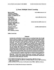
In  the  CMU  PIE  face  database  [17],  there  are  totally  68  people,  and  each  person  has  13  pose  variations  ranged  from  the  full  right  profile  image  to  the  full  left  profile  image  and  43  different  lighting  conditions,  21  flashes  with ambient light on or off. In our experiments, for each  person,  we  select  56  images  including  13  poses  with  neutral expression and 43 different lighting conditions in  the  frontal  view.  For  all  frontal‐view  images,  we  apply  alignment based on two eye center and nose center points,  and  no  alignment  is  applied  on  the  other  images  with  poses.  All  the  segmented  images  are  rescaled  to  the  resolution  of  92  ×  112,  and  then  reduced  to  wavelet  feature  faces  with  resolution  49×59  after  1‐level  Daubichies‐4 (Db4) wavelet decomposition. Some images  of one person are shown in Fig. 2. 

Xiao-Zhang Liu and Guo-Can Feng: Multiple Kernel Learning in Fisher Discriminant Analysis for Face Recognition

5

4.3 Recognition results  This section reports the recognition results of MKFD and  KDDA  with  single  kernels  on  the  FERET  and  the  CMU  PIE  datasets.  For  each  subject  in  the  FERET  dataset,  we  randomly  select  n  ( n  2  to  5)  out  of  6  images  for  training, with the rest for testing. In the CMU PIE dataset,  the  number  of  randomly  selected  training  images  is  ranged from 10 to 18 out of 56 for each individual, while  the  rest  are  testing  images.  The  average  recognition  accuracies  over  10  runs  on  the  FERET  and  CMU  PIE  datasets are shown in Fig. 4(a)‐(b), respectively.  

 

  Figure 2. Some images of one person from the CMU PIE face  database 

4.2 Distribution of extracted features  This  section  aims  to  provide  insights  on  how  the  proposed  MKFD  simplifies  the  face  pattern  distribution,  compared with KDDA based on single kernels, when the  patterns are subject to pose and illumination variations.    We  select  five  subjects,  56  images  per  subject,  with  varying  pose  and  illumination,  from  our  CMU  PIE  face  dataset  determined  above  (56× 5 ＝ 280  images  in  all).  Four  types  of  feature  bases  are  generalized  from  the  images  by  utilizing  KDDA  with  linear  kernel,  KDDA  with  Gaussian  RBF  kernel,  KDDA  with  polynomial  kernel,  and  our  MKFD,  respectively.  In  the  sequence,  all  the 280 images are projected onto the four subspaces. For  each  image,  its  projections  in  the  first  two  most  significant  feature  bases  of  each  subspace  are  visualized  in Fig. 3. 

 

a) Linear-kernel KDDA based subspace

b) RBF-kernel KDDA based subspace

c) Polynomial-kernel KDDA based subspace

d) MKFD based subspace

 

Fig.  3(a)‐(d)  depict  the  first  two  most  discriminant  features  extracted  by  utilizing  KDDA  with  linear  kernel,  KDDA  with  Gaussian  RBF  kernel,  KDDA  with  polynomial  kernel  and  MKFD,  respectively.  Obviously,  our MKFD extracts the most discriminant features. 

Int J Adv Robotic Sy, 2013, Vol. 10, 142:2013

Table 1 shows the average and standard deviation of the  accuracies  for  FERET  ( n  3:  3  images  per  subject  for  training  with  the  rest  for  testing)  and  CMU‐PIE  ( n  14:  14 images per subject for training with the rest for testing),  respectively.     FERET  CMU PIE  Type of kernel     (n=3)  (n=14)  Mean   84.94%   71.79%   Linear kernel   Std   0.015  0.014  RBF kernel  

Mean   Std  

73.84%   0.040  

69.03%   0.010  

Polynomial kernel  

Mean   Std  

84.80%   0.017 

76.50%   0.010 

Multi‐kernel with   same weights  

Mean   Std  

80.84%   0.030 

71.81%   0.014 

Multi‐kernel with   optimized weights  

Mean   Std  

86.34%   0.015 

78.74%   0.007 

Table 1. Performance comparison between MKFD and KDDA  with single kernels 

Figure 3. Distribution of 280 images of five subjects under  varying pose and illumination in four types of subspaces 

6

  Figure 4. Comparison of accuracies obtained by MKFD and  KDDA with single kernels  

From the results in Fig. 4 and Tables 1, it can be seen that,  the  blending  of  multiple  kernels  in  the  proposed  MKFD  can achieve higher accuracies than any of the three single  kernels,  but  a  simple  summation  of  multiple  kernels  is  hardly  a  good  idea  for  improving  the  classification  performance,  while  our  constructed  multiple  kernel  function  with  optimized  kernel  weights  leads  to  enhanced performance.    Note  that  in  the  experiments,  neither  the  parameter  for  RBF kernel nor the one for polynomial kernel is optimally  selected,  and  even  linear  kernel  has  no  parameter.  This 

www.intechopen.com

means  that,  to  a  certain  extent,  the  multiple  kernel  function  relaxes  parameter  selection  about  the  base  kernels.  5. Conclusion  In this paper, on the assumption that multiple kernels can  characterize  geometrical  structures  of  the  original  data  from  multiple  views  which  can  complement  to  improve  recognition  performance,  we  apply  kernel‐based  FDA  with  multiple  kernels,  which  we  call  MKFD,  to  recognition  of  face  images  under  variations  of  pose,  illumination,  facial  expression,  etc.  The  constructed  kernel  for  MKFD  is  a  linear  combination  of  several  base  kernels with a constraint on their weights. By maximizing  the  margin  maximization  criterion,  we  propose  an  iterative  scheme  based  on  the  method  of  Lagrange  multipliers  for  the  weight  optimization,  which  yields  updated  kernel  weights  resulting  in  high  recognition  accuracy  on  the  FERET  and  CMU  PIE  face  database,  compared  with  the  single  kernels.  The  experiments  also  demonstrate  that  the  multiple  kernel  function  relaxes  parameter selection to some extent.    It  is  important  to  point  out  that  the  proposed  weight  optimization  scheme  is  generic  and,  with  minor  modifications,  can  be  applied  to  all  kernel‐based  FDA  algorithms.  6. Acknowledgement  This work is partially supported by the National Natural  Science Foundation of China under grant No. 60975083.  7. References  [1] M. Turk and A. Pentland. Eigenfaces for recognition. J.  Cogn. Neurosci., 3(1):71–86, 1991.  [2] P. N. Belhumeur, J. P. Hespanha, and D. J. Kriegman.  Eigenfaces  vs.  Fisherfaces:  Recognition  using  class  specific  linear  projection.  IEEE  Trans.  Pattern  Anal.  Mach. Intell., 19(7):711–720, Jul. 1997.  [3]  A.  Ruiz  and  P.E.  López  de  Teruel.  Nonlinear  kernel‐ based  statistical  pattern  analysis.  IEEE Trans.  Neural  Netw., 12(1):16–32, Jan. 2001.  [4]  B.  Schölkopf,  A.  Smola,  and  K.Müller.  Nonlinear  component analysis as a kernel  eigenvalue  problem.  MPI  fur  biologische  kybernetik,  Tubingen,  Germany,  Tech. Rep. 44, 1996.       

www.intechopen.com

[5] S. Mika, G. Rätsch, J. Weston, B. Schölkopf, and K. R.  Müller.  Fisher  discriminant  analysis  with  kernels.  Proc.  IEEE  workshop  Neural  Netw.  Signal  Process.  IX,  1999, pp. 41‐48.  [6]  G.  Baudat  and  F.  Anouar.  Generalized  discriminant  analysis  using  a  kernel  approach.  Neural  Comput.,  12(10):2385‐2404, 2000.  [7]  J.  W.  Lu,  K.  Plataniotis,  and  A.  N.  Venetsanopoulos.  Face  recognition  using  kernel  direct  discriminant  analysis  algorithms.  IEEE  Trans.  Neural  Netw.,  14(1):117‐126, Jan. 2003.  [8]  O.  Chapelle,  V.  Vapnik,  O.  Bousquet,  and  S.  Mukherjee.  Choosing  multiple  parameters  for  support  vector  machines.  Machine  Learning,  46(1‐ 3):131‐159, 2002.  [9]  S.  Sonnenburg,  G.  Rätsch,  and  C.  Schäfer.  A  general  and  efficient  multiple  kernel  learning  algorithm.  Neural Information Processing Systems, 2005.  [10]  Z.  Wang,  S.  Chen,  and  T.  Sun.  MultiK‐MHKS:  A  novel multiple kernel learning algorithm. IEEE Trans.  Pattern Anal. Mach. Intell., 30(2):348‐353, Feb. 2008.  [11]  J.  Bi,  T.  Zhang,  and  K.  Bennett.  Column‐generation  boosting  methods  for  mixture  of  kernels.  Proc.  Int’l  Conf.  Knowledge  Discovery  and  Data  Mining,  pp.  521‐ 526, 2004.  [12]  G.R.G.  Lanckriet,  N.  Cristianini,  P.  Bartlett,  L.E.  Ghaoui, and M.I. Jordan. Learning the kernel matrix  with  Semidefinite  Programming.  J. Machine Learning  Research, vol. 5, pp. 27‐72, 2004.  [13]  F.  Bach,  G.R.G.  Lanckriet,  and  M.I.  Jordan.  Multiple  kernel learning, conic duality, and the SMO algorithm.  Proc. 21st Int’l Conf. Machine Learning, 2004.  [14]  K.P.  Bennett,  M.  Momma,  and  M.J.  Embrechts.  MARK:  A  boosting  algorithm  for  heterogeneous  kernel models. Proc. ACM SIGKDD, pp. 24‐31, 2002.  [15]  H.  Li,  T.  Jiang,  and  K.  Zhang.  Efficient  and  robust  feature  extraction  by  maximum  margin  criterion.  Advances in Neural Information Processing Systems 16, S.  Thrun,  L.  Saul,  and  B.  Schölkopf,  Eds.  Cambridge,  MA, MIT Press, pp. 157 ‐165, 2004.  [16]  P.  J.  Phillips,  H.  Moon,  S.  A.  Rizvi,  and  P.  J.  Rauss.  The  FERET  evaluation  methodology  for  face‐ recognition  algorithms.  IEEE  Trans.  Pattern  Anal.  Mach. Intell., 22(10):1090–1104, Oct. 2000.  [17]  T.  Sim,  S.  Baker,  and  M.  Bsat.  The  CMU  pose,  illumination, and expression (PIE) database. Proc. 5th  IEEE  Int.  Conf.  Autom.  Face  and  Gesture  Recogntion,  May 2002. 

Xiao-Zhang Liu and Guo-Can Feng: Multiple Kernel Learning in Fisher Discriminant Analysis for Face Recognition

7