More Efficiency in Multiple Kernel Learning - CiteSeerX

More Efficiency in Multiple Kernel Learning

Alain Rakotomamonjy [email protected] LITIS EA 4051, UFR de Sciences, Université de Rouen, 76800 Saint Etienne du Rouvray, France Francis Bach [email protected] CMM, Ecole des Mines de Paris, 35 rue Saint-Honoré, 77305 Fontainebleau, France St´ ephane Canu LITIS EA 4051, INSA de Rouen, 76801 Saint Etienne du Rouvray, France

[email protected]

[email protected]

Yves Grandvalet IDIAP, Rue du Simplon 4, Case Postale 592, CH-1920 Martigny, Switzerland

Abstract An efficient and general multiple kernel learning (MKL) algorithm has been recently proposed by Sonnenburg et al. (2006). This approach has opened new perspectives since it makes the MKL approach tractable for largescale problems, by iteratively using existing support vector machine code. However, it turns out that this iterative algorithm needs several iterations before converging towards a reasonable solution. In this paper, we address the MKL problem through an adaptive 2-norm regularization formulation. Weights on each kernel matrix are included in the standard SVM empirical risk minimization problem with a `1 constraint to encourage sparsity. We propose an algorithm for solving this problem and provide an new insight on MKL algorithms based on block 1-norm regularization by showing that the two approaches are equivalent. Experimental results show that the resulting algorithm converges rapidly and its efficiency compares favorably to other MKL algorithms.

regression (Scholkopf & Smola, 2001). For such tasks, the performance of the learning algorithm strongly depends on the data representation. In kernel methods, the data representation is implicitly chosen through the so-called kernel K(x, x0 ). This kernel actually plays several roles: it defines the similarity between two examples x and x0 , while defining an appropriate regularization term for the learning problem. For kernel algorithms, the solution of the learning problem is of the form: f (x) =

Appearing in Proceedings of the 24 th International Conference on Machine Learning, Corvallis, OR, 2007. Copyright 2007 by the author(s)/owner(s).

αi? yi K(x, xi ) + b? ,

(1)

i=1

where {xi , yi }ì=1 are the training examples, ` the number of learning examples, K(·, ·) is a given positive definite kernel associated with a reproducing kernel Hilbert space (RKHS) H and {αi? }i , b? some coefficients to be learned from examples. Recent applications (Lanckriet et al., 2004a) and developments based on SVMs have shown that using multiple kernels instead of a single one can enhance interpretability of the decision function and improve classifier performance. In such cases, a common approach is to consider that the kernel K(x, x0 ) is actually a convex linear combination of other basis kernels:

1. Introduction During the last few years, kernel methods, such as support vector machines (SVM) have proved to be efficient tools for solving learning problems like classification or

` X

K(x, x0 ) =

M X

k=1

dk Kk (x, x0 ), with dk ≥ 0,

X

dk = 1,

k

where M is the total number of kernels. Each basis kernel Kk may either use the full set of variables describing x or only a subset of these variables. Alternatively, kernels Kk can simply be classical kernels (such as Gaussian kernel) with different parameters,


or may rely on different data sources associated with the same learning problem (Lanckriet et al., 2004a). Within this framework, the problem of data representation through the kernel is then transferred to the choice of weights dk . Learning both the coefficients αi and the weights dk in a single optimization problem is known as the multiple kernel learning (MKL) problem. This problem has been recently introduced by Lanckriet et al. (2004b) and the associated learning problem involves semi-definite programming which makes the problem rapidly intractable as the number of learning examples or kernels become large. Bach et al. (2004) have reformulated the problem and then proposed a SMO algorithm for medium-scale problems. Another formulation of this problem based on a semi-infinite linear problem (SILP) has been proposed by Sonnenburg et al. (2006). The advantage of this latter formulation is that the algorithm solves the problem by iteratively solving a classical SVM problem with a single kernel (for which many efficient toolboxes exist) and a linear programming for which number of constraints increases along with iterations. In this paper, we present another formulation of the multiple learning problem. We first depart from the framework proposed by Bach et al. (2004) and further used by Sonnenburg et al. (2006). Indeed, instead of using a 1-norm block regularization, we propose, in Section 2, a weighted 2-norm regularization of each function induced by the kernel Kk ; we control the sparsity of the linear combination of kernels, by adding a 1norm regularization constraint on these kernel weights. This adaptive multiple kernel regularization can then be solved through an iterative algorithm as described in Section 2.2, by means of a standard SVM implementation and a gradient descent procedure. A side contribution of this paper is to offer another insight to the work of Bach et al. (2004). Indeed, following the line of Grandvalet (1998), by using a variational formulation of the 1-norm block regularization, we show that the two formulations are equivalent (see Section 3.1). Furthermore, we discuss the convergence properties of our algorithm in Section 3.4. After these developments, we present an experimental section that illustrates the efficiency of our algorithm and some concluding remarks.

2. Multiple Kernel Learning Framework We present in this section the formulation of our multiple kernel learning problem and the algorithm we propose for solving it. In order to simplify notations, in the sequel, all summation on i and j goes from 1 to `, while summation on k goes from 1 to M .

2.1. Problem Formulation We consider the classification learning problem from data {xi , yi }ì=1 where xi belongs to some input space X and yi = {+1, −1} denoting the class label of examples xi . In the support vector machines methodology, the decision function is of the form given in equation (1) where the optimal vector αi? and real b? are obtained by solving the dual of the following optimization problem : minf ∈H,b∈R with

1 2 i ξi 2 kf kH + C yi (f (xi ) + b) ≥ 1 − ξi

ξi ≥ 0

∀i

P

∀i

In some situations, a machine learning practitioner may be interested in another form of decision function. For instance, in the so-called multiple kernel learning framework,P he looks for a decision function of the form f (x)+b = k fk (x)+b with each fk ∈ Hk where Hk is the RKHS associated with kernel Kk . Inspired by the multiple smoothing splines framework (Wahba, 1990), the approach we propose in this paper for solving this multiple kernel SVM problem is based on the resolution of the following problem : P P 1 2 mindk ,fk ,b,ξi i ξi k dk kfk k + C P f (x ) + y b ≥ 1 − ξi ∀i with yP k i i i k (2) d = 1 k k ξi ≥ 0, dk ≥ 0 ∀i, ∀k where each dk controls the squared norm of fk in the objective function. Hence the smaller dk is, the smoother fk should be. When dk = 0, we will prove in the sequel that fk must also be equal to zero, so that the problem stays well-defined. Note that a sparsity constraint of the vector d has been added through a `1 norm constraint and then it should lead to a sparse decision function with few basis kernels. Note that the function to be minimized is jointly convex in its parameters d, {fk }, b, and ξ. 2.2. Solving the Problem One possible approach for solving the problem given in equation (2) is to use a 2-step alternate optimization algorithm, followed for example by Grandvalet and Canu (2003) in a different context. The first step would consist in solving problem (2) with respect to fk , b and ξ while considering that the vector d is fixed. Then, the second step consists in updating the weight vector d through a descent step towards the minimum of the objective function of equation (2) for fixed fk , b and ξ. In Section 3.1 we show that the second term can be computed in closed form. However, such an


approach does not always have convergence guarantees and may lead to numerical problems, in particular when one dk approaches zero (Grandvalet, 1998). In some other cases, it is possible to have a convergence proof of such alternate optimization algorithm (Argyriou et al., 2007). Instead, we prefer to consider the problem as the following constrained optimization problem : PM (3) mind J(d) such that k=1 dk = 1, dk ≥ 0 where

  minfk ,b,ξi J(d) = with 

1 2

1 2 dk kfk k

P + C i ξi yi k fk (xi ) + yi b ≥ 1 − ξi ξi ≥ 0 P Pk

(4)

The objective function J(d) is actually an optimal SVM objective value. We solve the minimization problem (3) on the simplex by means of a projected gradient method, which assumes that J(·) is differentiable and requires the computation of its gradient. 2.2.1. Computing J(·) and its Derivatives First, we show that for a given vector d, J(d) is the objective value of a classical P SVM problem where the kernel is : K(xi , xj ) = k dk Kk (xi , xj ). Then, under some reasonable conditions, we show that J(d) is differentiable. Indeed, the Lagrangian of the primal problem (4) can be written : L =

X 1X 1 ξi kfk k2 + C 2 dk i k X X X + αi (1 − ξi − yi ( fk (xi ) + b)) − νi ξi i

k

i

and setting the derivatives of this Lagrangian according to the primal variables to zero gives : P (a) d1k fk (·) = i αi yi Kk (·, xi ), ∀k P (5) (b) i αi yi = 0 (c) C − αi − νi = 0, ∀i According to these equations, the associated dual problem is : P P P maxα − 21 i,j αi αj k dk Kk (xi , xj ) + i αi P with i αi yi = 0 C ≥ αi ≥ 0 (6) This is the usual SVM dual P problem using a single kernel matrix K(xi , xj ) = k dk Kk (xi , xj ). Hence, this step can be solved by any SVM algorithm. The more

efficient this SVM algorithm is, the more efficient our MKL algorithm becomes. Furthermore, If this SVM algorithm is able to handle a large-scale problem, then this MKL algorithm can also solve large-scale problem. Thus, the overall complexity of our MKL algorithm is tied to the one of the single kernel SVM algorithm. Also note that according to the Lagrangian derivatives, fk (·) goes to 0 as the coefficient dk vanishes. For computing the derivatives of J with respect to d, let us note that J(d) is the optimal objective value of equation (4) solved above. and J(d) can be seen as an implicit function. Then for a given d, because of strong duality, J(d) is also the objective value of the dual problem. Then, we also have : J(d) = −

X 1 X ? ?X αi αj dk Kk (xi , xj ) + αi? 2 i,j i k

where the vector α? optimizes equation (6). We assume for the rest of the paper that each kernel matrix (Kk (xi , xj ))i,j has a minimal eigenvalue greater than a fixed small η > 0 (if the original kernels do not verify this, a small rigde may be added on the diagonal of the kernel matrices). This implies that the dual function is strictly concave with convexity parameter η (Lemaréchal & Sagastizabal, 1997). Differentiability issues and derivatives computation of optimal values of optimization problems have been largely discussed by Bonnans and Shapiro (1998). The particular case of SVM have been addressed by Chapelle et al. (2002). From these works, we know that J(d) is differentiable if the SVM solution is unique. This unicity is ensured by the strict concavity of the dual function. And in such cases, derivatives of J(d) can be computed as if the optimal value of α? does not depend on dk . Thus, by simply derivating the dual function given in equation (6) wrt to dk , we have : 1X ? ? ∂J =− α α yi yj Kk (xi , xj ) ∂dk 2 i,j i j

∀k

(7)

2.2.2. Algorithm The optimization problem we have to deal with is a non-linear optimization with linear constraints (see equation (3)). With our positivity assumption on the kernel matrices, J(·) is convex, differentiable with Lipschitz gradient (Lemaréchal & Sagastizabal, 1997). The approach we used for solving such problem is then a projected gradient method, which does converge for such functions (Bonnans et al., 2003). Once the gradient of J(d) has been computed, d is


Algorithm 1 adaptive 2-norm multiple kernel algorithm 1 d1k = M for k = 1, · · · , M for t = 1, 2, · · · do solve P t the classical SVM problem with K = k d k Kk ∂J compute ∂d for k = 1, · · · , M k compute descent direction Dt and optimal step γt ← dtk + γt Dt,k dt+1 k if stopping criterion then break end if end for

updated by gradient descent while ensuring that the constraints on d are satisfied. This can be done first by reducing the gradient and then by projecting the gradient so that non-negativity of d is ensured. In other words, the updating scheme will be the following :

optimization problem: P P 2 minwk ,b,ξi 21 (P k kwk k) + C i ξi with yi k hwk , Φk (xi )i + yi b ≥ 1 − ξi ξi ≥ 0

where Φk (x) is a non-linear mapping of x to a RKHS Hk . What makes this formulation interesting is that the `1 -norm block penalization of wk leads to a sparse solution in w and thus, the algorithm automatically performs kernel selection. We have stated in the previous section that our algorithm also performs some kind of kernel selection by weighting each squared-norm of fk and by adding a `1 norm constraints on these weights. We show in the following that these two formulations (Bach et al.’s and ours) are equivalent. At first, equation (8) formulation can be rewritten in the following functional form : minfk ,b,ξi with

dt+1 ← dt + γt Dt where Dt is the vector of descent direction. The step size γt is determined by using a one-dimensional line search, with proper stopping criterion such as Armijo’s rule, which ensures global convergence. Note that the line-search technique involves querying the objective function and thus needs the computation of several single kernel SVM with small variations of d. However, this part can be speeded up by initializing the SVM algorithm with previous values of α? . The overall algorithm is described in Algorithm 1. We can see that the above described steps are performed until a stopping criterion is met. This stopping criterion can be either based on a duality gap, or more simply, on a maximal number of iterations, or on the variation of d between two consecutive steps.

P P 2 1 i ξi 2 (P k kfk k) + C yi k fk (xi ) + yi b ≥ 1 − ξi

(9)

ξi ≥ 0

In order to prove the equivalence of both formulation, we simply show that the variational formulation of the 1-norm block regularization is equal to the adaptive weighted 2-norm regularization, (which is a particular case of a more general equivalence proposed by Micchelli and Pontil (2005)) i.e :

min P

dk ≥0,

k

dk =1

X kfk k2 dk

k

=

X k

!2

kfk k

(10)

For proving this equality, we use a classical Lagrangian approach. Hence, the Lagrangian of the primal is : ! X X kfk k2 X L= dk − 1 − +ν ηk dk dk k

k

3. Discussions

At optimality, we have :

In this section we discuss the connection of our multiple kernel learning framework with other multiple kernel algorithms (and their equivalence) and address other points like computational complexity, extensions to other SVM algorithms and convergence of the algorithm.

(a) d2k =

kfk k2 , ∀k ν − ηk

(b)

X

k

dk = 1

k

(c) ηk dk = 0, ∀k

(11) according to (c), we can state for all k that√ either kfk k = 0 and thus dk = 0 or dk = kfk k/ ν and ηk = 0. Then at optimility, we have : X kfk k2

3.1. Connections with 1-norm Block Regularization Formulation of MKL The multiple kernel learning formulation introduced by Bach et al. (2004) and further developed by Sonnenburg et al. (2006) consists in solving the following

(8)

k

dk P

=

√ X ν kfk k k

√ with k dk = 1 = k kfk k/ ν which proves the variP 2 ational formulation of ( k kfk k) given in equation (10). P


This proof shows that the non-smooth 1-norm block regularized optimization original problem has been turned into a smooth (under positive definiteness conditions) optimization problem at the expense of adding variables. However, although the number of variables has increased, we will see that this problem can be solved more efficiently. 3.2. Computational Complexity We can note that the algorithm of Sonnenburg et al. (2006) and ours are rather similar since they are both based on the MKL algorithm wrapped around a single SVM algorithm. This makes both algorithms very easy to implement and efficient. The main difference between the two algorithms resides in how the kernel weights dk are optimized. The algorithm of Sonnenburg et al. (2006) uses a linear programming involving M variables and an increasing number of constraints, which is equivalent, as shown in Section 3.5, to a cutting plane method. Our algorithm is based on a gradient descent procedure involving a reduced gradient technique. Although the overall complexity of our algorithm is difficult to evaluate formally, we can have some clues about it. For each iteration, our algorithm needs one single kernel SVM formulation and the computation of the gradient of J(d). The gradient computation have a complexity of the order of n3SV · M , where nSV is the number of non-zeros alpha’s at that given iteration. The main burden involved in the projected gradient technique is the several SVM retrainings. The number of these retrainings is data and step dependent however since we use a good initialization of the SVM, this step is rather cheap.

same as for 2-class SVM. Hence, the structure of the algorithm does not change, except for the calculation of the step size since it needs the computation of the dual objective value. 3.4. Convergence Analysis In this paragraph, we briefly discuss the convergence of the algorithm we propose. We first suppose that problem (4) is always exactly solved, which means that the duality gap of such problem is 0. With such conditions, our gradient computation in equation (7) and thus our algorithm is performing steepest projected gradient descent on a continuously differentiable function J(·) (remember that we have assumed that the kernel matrices P are positive definite) defined on the simplex {d, k dk = 1, dk ≥ 0}, which does converge to the global minimum of J (Bonnans et al., 2003). However, in practice, problem (4) is never solved exactly since most SVM algorithm will stop when the duality gap is smaller than a certain ε. In this case, the convergence of our projected gradient method is no more guaranteed by standard arguments. Indeed, the output of the approximately solved SVM leads only to an ε-subgradient (Bonnans et al., 2003; Bach et al., 2004). This situation is more difficult to analyze and we plan to address it completely in future work. 3.5. Cutting Planes vs. Steepest Descent Our differentiable function J(d) is defined as:    1X X X  dk Kk (xi , xj ) + αi αj αi J(d) = max − α  2  i,j i k

3.3. Extensions to other SVM Algorithms In this paper we have focused on the SVM algorithm for binary classification, but it is worth noting that our multiple kernel learning algorithm can be extended to other SVM algorithms without much effort. However, since this point is not the main focus of the paper, we simply sketch the outline of these extensions here. For another algorithm, say one-class SVM, the change would be merely the loss function and thus the definition of J(d) in problem (4). Then, for the algorithm, the first step would simply consists P in optimizing a oneclass SVM with a kernel K = k dk Kk while for the second step the gradient of the objective function according to dk is needed. Hence, the main effort for the extension has to be devoted to the processing of this gradient through the dual of the 1-class SVM problem. In this particular case, the gradient of J would be the

The SILP algorithm of Sonnenburg et al. (2006) is exactly equivalent to a cutting plane method to minimize the function J. Indeed, for each value of d, the best α is found and leads to an affine lower bound on J(d). As more d’s and α’s are computed, the number of lower bounding affine functions increases and the next vector d is found as the minimizer of the maximum of all those affine functions. Cutting planes method do converge but they are known for their instability, notably when the number of lower-bounding affine functions is small (Bonnans et al., 2003): the approximation of the objective function is then loose and the iterates may oscillate, as shown in Section 4. In this paper, we use a steepest descent approach which does not suffer from instability issues since we have a differentiable function to minimize.


4. Numerical Experiments

1 0.8

dk

0.6 0.4 0.2 0

0

10

20

30

40

50

60

70

80

90

100

1 0.8 0.6

dk

We apply our multiple kernel learning algorithm to real-world datasets coming from the UCI repository : Liver, Credit, Ionosphere, Pima, Sonar. For the multiple kernels, we have used a Gaussian kernel with 10 different bandwidths σ, on all variables and each single variable. We have also used a polynomial kernel of degree 1 to 3 again on all and each single variable. Note that in all the experiments, kernel matrices have been precomputed prior to running the algorithm. Kernels have also been normalized to unit trace.

0.4 0.2 0

1

2

3

4

5

6

7

8

Iterations 0.06

0.04

Difference of dk

0.02

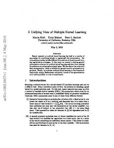
We have compared our algorithm to the SILP approach of Sonnenburg et al. Both algorithms use a SVM dual solver based on an active constraints method written in Matlab. The linear programming involved in the SILP approach has been solved using the publicly available toolbox LPSOLVE. The gradient descent procedure of our algorithm has been implemented in Matlab. While running our algorithm, a coefficient dk smaller than 0.001 is forced to 0. All the experiments have been run on a Pentium D-3 GHz and 1GB of RAM. For a fair comparison, we have selected the same termination criterion for these iterative algorithms : iteration terminates when ||dt+1 − dt ||∞ < 0.01 or the maximal number of iteration (500) has been reached. For each dataset, we have run both algorithms 50 times with different training and testing splits (50 % of all the examples for training and testing). Training sets have been normalized to zero mean and unit variance and the test sets have also been rescaled accordingly. Different values of the hyperparameter C (0.1, 1, 10, 100) have been tried. In Table 1, we have reported different performance measures of both algorithms only for the values of C that leads to the best accuracy performance. Although, this procedure is unusual since it does not take into account a proper model selection procedure, this is relevant since we are essentially interested in other performance measures such as the number of kernels selected or the running time. Results in Table 1 show that both algorithms are comparable in performance accuracy. The main differences we observe rely on the number of kernels selected by both algorithms and their running time. We can see that our algorithm tends to select a larger number of kernels. A rationale for this observation can be the following. For our algorithm, the update of dk is based on a gradient descent algorithm. Hence, due to slow convergence of given coefficient towards 0, the termination criterion we choose may stop the algorithm too early.

0

−0.02

−0.04

−0.06

−0.08

0

20

40

60

80

100

120

Index of kernels

Figure 1. Example of evolution and final values of the coefficients dk weighting the kernels for the SILP algorithm and our adaptive 2-norm algorithm. This figure has been obtained for Pima dataset and C = 100. (top) Evolution of dk for the SILP algorithm. (middle) Evolution of dk for our adaptive 2-norm regularization algorithm. (bottom) Difference of the final values of dk of the 2 algorithms R dSILP − dOU (117 kernels have been used). k k

The main advantage of our algorithm is the computational time needed for convergence of the algorithm. On all the datasets we used, our algorithm is faster than the one of Sonnenburg’s et al. This difference in running time can be understood from Figure 1. This figure illustrates the behavior of the dk coefficients as the iteration increases. One one hand, we can see that the SILP algorithm spends many iterations before converging towards a reasonable solution of dk . Hence, as stated by Sonnenburg et al (Sonnenburg et al., 2006), many SVM trainings are unnecessarily costly since the dk are still far away from optimal. On the other hand, our algorithm converges after fewer iterations, although the solution is not strictly equal to the one obtained with SILP, as we can see on the right side of the Figure (the convex optimization problems are solved with a small but non zero duality gap, so solutions may actually slightly differ). 4.1. Computing Approximate Regularization Paths In the previous experiment, we have compared the performances and running time of the MKL SILP algorithm and our algorithm for a single value of C. How-

More Efficiency in Multiple Kernel Learning Table 1. Some performance measures of the two MKL algorithms. For the best hyperparameter C value, we have averaged over 50 trials the number of kernels selected, average accuracy of the resulting decision function and the running time. The number of kernels M is also given.

Liver M = 91 # Kernel Accuracy 8.3 ± 1.8 65.4 ± 2.7 10.2 ± 2.0 65.0 ± 2.3

Time (s) 7.7 ± 2.7 3.2 ± 0.9

Algorithm SILP Our

Pima M = 117 # Kernel Accuracy 10.9 ± 1.6 75.8 ± 1.8 14.3 ± 2.2 75.8 ± 1.6

Time (s) 78.0 ± 18.8 27.1 ± 7.2

Algorithm SILP Our

Credit M = 208 # Kernel Accuracy 10.4 ± 1.9 86.4 ± 1.4 16.8 ± 5.4 86.3 ± 1.4

Time (s) 124 ± 28 32.7 ± 9.7

Algorithm SILP Our

Ionosphere M = 442 # Kernel Accuracy 19.9 ± 2.1 92.2 ± 1.5 30.5 ± 7.0 92.3 ± 1.4

Time (s) 152 ± 39 18.1 ± 5.8

Algorithm SILP Our

Sonar M = 793 # Kernel Accuracy 29.1 ± 3.5 79.2 ± 4.6 46.0 ± 7.6 78.6 ± 4.2

Results on the running time of both algorithms for computing the approximate regularization paths are given in Figure 3 and Table (2). They have been obtained by averaging 5 runs over different training sets. Figure 3 plots the computational time for each value of C. Since C = 100 is the initial state of the algorithm, no warm-start has been used, hence the large running time value. We can see that for the SILP MKL algorithm, the computational time is somewhat linear with C, whereas using the adaptive 2-norm algorithm, the running time rapidly decreases ( when decreasing C from 100) and then reaches a steady state with small computational time. Table 2 depicts the average time (over 5 runs) for computing the whole approximate regularization path with 100 samples of C. We can note that our adaptive 2-norm algorithm is more efficient than SILP and that the gain factor goes from 5 to 66. This gain factor is better when the number of kernels is large. 1 0.8 0.6

dk

Algorithm SILP Our

involved in the decision function when C is large and when C is small, only a single (or few) kernel tends to be selected. This finding is consistent over the datasets we used.

0.4 0.2 0

0

10

20

30

40

50

60

70

80

90

100

60

70

80

90

100

C 1 0.8 0.6

dk

Time (s) 383 ± 113 21.8 ± 16.9

0.4 0.2 0

ever, in many applications, this optimal value of is unknown and usually, one has to compute several decision functions with varying C and then choose the optimal one according to some model selection criterion like the cross-validation error. In this other experiment, we have evaluated the running time of both algorithms when C is varying and when using a warm-start technique. In our case, a warm-start approach (DeCoste & Wagstaff., 2000) consists in using the optimal solutions {dk } and αi? obtained for a given C to initialize a new MKL problem with C + ∆C. In our case, we have started with the largest value of C and then we have followed the regularization path by decreasing C. The experimental setup is the same as the previous one. Furthermore, we have consider 100 values of the hyperparameter C. We have sampled 50 values of C in both intervals [0.1, 10] and [10, 100]. Figure 2 gives an example of the regularization path of d with varying C. We can note for instance that there is more kernels

0

10

20

30

40

50

C

Figure 2. Approximate regularization paths of the dk with respects to C for the Ionosphere dataset. Each solution, except for C = 100, has been computed using a warmstart techniques and with decreasing C. (top) Adaptive two-norm MKL. (bottom) SILP MKL.

5. Conclusion In this paper, we have introduced another approach for solving the multiple kernel learning problem in support vector machines. Our approach uses an weighted 2-norm regularization while imposing sparsity on the weights. Hence, our algorithm is able to perform kernel selection. We have also showed that a solution of our algorithm is also a solution of the multiple kernel problem introduced by Bach et al. (2004), making the two algorithms equivalent in this sense. In the experiments, we have illustrated that our algorithm gives equivalent accuracy performance results while select-

More Efficiency in Multiple Kernel Learning 180

Bach, F., Lanckriet, G., & Jordan, M. (2004). Multiple kernel learning, conic duality, and the smo algorithm. Proceedings of the 21st International Conference on Machine Learning (pp. 41–48).

SILP adapt

160

140

Time (s)

120

100

80

Bonnans, J., Gilbert, J., Lemaréchal, C., & Sagastizbal, C. (2003). Numerical optimization theoretical and practical aspects. Springer.

60

40

20

0

0

10

20

30

40

50

60

70

80

90

100

C

Figure 3. Averaged over 5 runs of each step computation time for both algorithms for the Ionosphere dataset. For C = 100, we have the largest computation time since in such case there is no warm-start.

Table 2. Averaged time computation (in seconds) of an approximated regularization path with 100 samples of C varying from 0.1 to 100. We compare the performance of the MKL SILP algorithm and our algorithm.

data Liver Pima Credit Ionosphere Sonar

SILP 612 ± 180 4496 ± 730 4830 ± 754 5000 ± 788 11234 ± 2928

Adaptive 116± 19 754 ± 44 753± 64 221 ± 22 170 ± 25

Ratio 5.3 6.0 6.4 22.6 66.1

ing more kernels than the SILP MKL algorithm. However, we have empirically showed that our algorithm is more stable in the kernel weights and thus it needs fewer iterations to converge towards a reasonable solution, making it globally faster than the SILP algorithm. Future works aim at improving both speed and sparsity in kernels of the algorithm (for instance by initializing the SILP framework with the results of our algorithm) and by extending this algorithm to other SVM algorithm such as the one-class or the regression SVM.

Acknowledgments We wish to thank reviewers for their useful comments. This work was supported by grants from the IST programme of the European Community under the PASCAL Network of excellence, IST-2002-506778.

References Argyriou, A., Evgeniou, T., & Pontil, M. (2007). Convex multi-task feature learning (Technical Report).

Bonnans, J., & Shapiro, A. (1998). Optimization problems with pertubation : A guided tour. SIAM Review, 40, 202–227. Chapelle, O., Vapnik, V., Bousquet, O., & Mukerjhee, S. (2002). Choosing multiple parameters for SVM. Machine Learning, 46, 131–159. DeCoste, D., & Wagstaff., K. (2000). Alpha seeding for support vector machines. International Conference on Knowledge Discovery and Data Mining. Grandvalet, Y. (1998). Least absolute shrinkage is equivalent to quadratic penalization. ICANN’98 (pp. 201–206). Springer. Grandvalet, Y., & Canu, S. (2003). Adaptive scaling for feature selection in svms. Advances in Neural Information Processing Systems. MIT Press. Lanckriet, G., Bie, T. D., Cristianini, N., Jordan, M., & Noble, W. (2004a). A statistical framework for genomic data fusion. Bioinformatics, 20, 2626–2635. Lanckriet, G., Cristianini, N., Ghaoui, L. E., Bartlett, P., , & Jordan, M. (2004b). Learning the kernel matrix with semi-definite programming. Journal of Machine Learning Research, 5, 27–72. Lemaréchal, C., & Sagastizabal, C. (1997). Practical aspects of moreau-yosida regularization : theoretical preliminaries. SIAM Journal of Optimization, 7, 867–895. Micchelli, C., & Pontil, M. (2005). Learning the kernel function via regularization. Journal of Machine Learning Research, 6, 1099–1125. Scholkopf, B., & Smola, A. (2001). Learning with kernels. MIT Press. Sonnenburg, S., Raetsch, G., Schaefer, C., & Scholkopf, B. (2006). Large scale multiple kernel learning. Journal of Machine Learning Research, 7, 1531–1565. Wahba, G. (1990). Spline models for observational data. Series in Applied Mathematics, Vol. 59, SIAM.