Multiple Outliers Detection Procedures in Linear ... - Eprint UTM

Matematika, 2003, Jilid 19, bil. 1, hlm. 29–45 c

Jabatan Matematik, UTM.

Multiple Outliers Detection Procedures in Linear Regression Robiah Adnan & Mohd Nor Mohamad Department of Mathematics University of Teknology Malaysia 81300 Johor Bahru Johor, Malaysia Halim Setan Faculty of Geoinformation Science and Engineering University of Teknology Malaysia 81300 Johor Bahru Johor, Malaysia Abstract This paper describes a procedure for identifying multiple outliers in linear regression. This procedure uses a robust fit which is the least of trimmed of squares (LTS) and the single linkage clustering method to obtain the potential outliers. Then multiple-case diagnostics are used to obtain the outliers from these potential outliers. The performance of this procedure is also compared to Serbert’s method. Monte Carlo simulations are used in determining which procedure performed best in all of the linear regression scenarios. Keywords: Multiple outliers, linear regression, robust fit, Least trimmed of squares, single linkage. Keywords Multiple outliers, linear regression, robust fit, least trimmed of squares, single linkage. Abstrak Kertas kerja ini menghuraikan satu prosedur untuk mengenalpasti gandaan data terpenncil dalam regresi linear. Prosedur ini menggunakan kaedah penyesuan teguh iaitu kaedah kuasa dua trim terkecil dan kaedah berkelompok pautann tunggal untuk mengecam data terpencil yang mungkin. Kemudian, diagnostik kes berganda digunakan untuk mengenalpasti data terpencil. Prestasi prosedur ini dibandingkan dengan Serbert. Simulasi Monte Carlo digunakan untuk mengenalpasti prosedur yang terbaik dalam semua keadaan regresi linear. Katakunci data terpencil berganda, regresi linear, penyesuain teguh, kuasa dua trim terkecil, pautan tunggal.

Robiah Adnan, Halim Setan & Mohd Nor Mohamad

30

1

Introduction

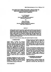
The linear regression model can be expressed in terms of matrices as y = Xβ +  where y is the n × 1 vector of observed response values, X is n × p matrix of p regressors (design matrix), β is the p × 1 regression coefficients and  is the n × 1 vector of error terms. The most widely used technique to find the best estimates of β is the method of ordinary least squares (OLS) which minimizes the sum of squared distances for all points from the actual observation to the regression surface. When the error terms are not normally and independently distributed (NID), distortion of the fit of the regression model can occur and consequently the parameter estimates and inferences can be flawed. The presence of one or more outliers is one of the common causes of non-normal error terms. As defined by Barnett and Lewis (1994), outliers are observations that appear inconsistent with the rest of the data set. Such outliers can have a profound destructive influence on the statistical analysis. It is not unusual to find an average of 10% outlying observations in data set of some processes (Hampel et al., 1986). Figure 1 illustrates the different types of outliers. The ellipse defines the majority of the data. Points A, B, and C are outliers in Y-space because their y values ( or response values) are significantly different from the rest of the data and they are also residual outliers (do not conform to the regression line or sometimes called regression outliers). Points B and C and D are outliers in X-space, that is, their x values are unusual and these are also referred to as leverage points. Although D is outlying in X-space, it is not a residual outlier. Points B and C are leverage points and residual outliers. Point A is an inlier in X-space but a residual outlier. Point E is an inlier in Y-space and also a residual outlier. All these different types of outliers can be summarized as in Table 1. Table 1: Different Types of Outliers Points A B C D E

Y-space outlier * * * * -

X-space outlier * * * *

residual outlier * * * *

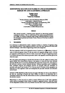
Figure 2 clearly indicates that it is of interest to regression practitioners to have a set of tools to detect outlying observations since with the presence of even two outlying observations, the estimates of the parameters can be significantly affected. It can be seen that the group of two outlying observations exerts a considerable influence on the least squares regression line and forces a fit of the data that is not representative of the majority of the data. Therefore using the least squares model to explain the relationship between the regressor and the response variable is inappropriate in the presence of outliers. For illustration, a hypothesized data set of size 20 where 2 of the observations are xy-space outlying is used in Figure 2. It is quite obvious that the dotted line in Figure 2 is of a better regression line for the data set used without taking the two outlying observations into consideration.

Multiple Outliers Detection Procedures in Linear Regression

31

Figure 1: Scatter plot for the different type of outlying observations Fortunately, isolating a single or a few outliers can be done quite easily using routine single-case diagnostics, that is, for example the Cook’s squared distance (Cook.,1979) measures the change in the regression coefficients that would occur if a case was omitted. But as can be seen in Figure 2, the ordinary least squares (OLS) estimates and inference can be affected with the presence of even two outliers. However , the standard single-case diagnostic measures often suffers from masking and swamping. Masking is the inability of the procedure to detect the outliers, while swamping is the detection of clean observations as outliers. It is generally agreed that there is no single multiple outlier identification procedure that can tackle all kinds of outliers scenarios. The modification of the procedure proposed by Serbert, et. al (1998) is of interest in this research. Serbert uses the least squares to fit the data and then cluster the data using single linkage by taking the standardized predicted values and residual values as the values in the calculation of the similarity measures. Since the proposed method (Method 1) uses the idea of a robust fit and clustering technique, therefore a brief description of these two ideas are given in sections 1.1 and 1.2 respectively. Section 1.3 describes the Monte Carlo simulation used in this research to evaluate the effectiveness of the proposed procedure in detecting multiple outliers. Section 1.4 discusses the multiple-row influence diagnostics which will be used in determining the ”true” outliers from the potential outliers obtained from Method 1.

1.1

Robust Fit /Robust Regression

This approach tries to devise estimators so that the regression fit will not be so strongly affected by outliers. From this robust fit the outliers may be identified by looking at the residuals. There are many such robust estimators in the literature but the least trimmed of squares (LTS) is of interest in this paper. One of the most important properties for robust regression estimators is breakdown point. Breakdown point is defined as the smallest fraction of unusual data that can cause the estimator to be useless. It is a well known fact that the LTS is a high breakdown estimator, that is, it can have a value of 50% which is the highest value possible (Rousseeuw and Leroy, 1987). Therefore the proposed Method 1 uses the standardized predicted values and residual values from the least trimmed of squares

32

Robiah Adnan, Halim Setan & Mohd Nor Mohamad

Figure 2: The OLS regression for a hypothesized data set of size 20 with two XY-space outlying observations

Multiple Outliers Detection Procedures in Linear Regression

33

(LTS) fit rather than the OLS fit . Figure 5 shows the least square fit and the LTS fit for a data set with outliers. From this graph it is obvious that the fit from the LTS is better compared to the OLS in the presence of outliers.

1.2

Clustering

The objective of cluster analysis is to find natural groupings of items ( or variables). The items in the resulting clusters should exhibit a high internal homogeneity and low external homogeneity. Clustering techniques can be divided into two groups: hierarchical and nonhierarchical. Hierarchical clustering techniques proceed by either a series of successive mergers, that is, starts with n clusters and end up with a cluster which contains all of the data points ( known as agglomerative hierarchical methods) or by a series of divisions, that is, starts with one cluster and end up with n clusters with each cluster containing one data point ( known as divisive hierarchical methods). An example of an agglomerative hierarchical method is the single linkage which is incorporated in Method 1. The single linkage algorithm uses the smallest distance between a point in the first cluster and a point in the second cluster. The distance between these two clusters can be shown graphically as below (Figure 3).

Figure 3: Single linkage

1.3

Monte Carlo Simulation

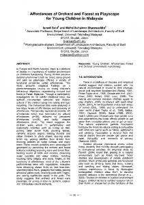
There are six outlier scenarios and a total of twenty four different situations considered in this research ( see Table 2). These scenarios are similar to those used by Serbert et al. (1998). The factors considered in this simulation are (1) levels of percentage of outliers: 10% or 20%, (2) number of outlying groups : one or two groups, (3) number of regressors : 1, 3, or 6 and (4) distances of outliers from clean observations : 5 standard deviations or 10 standard deviations. There are 1000 replications for each scenario and all simulations are done in S-Plus version 4.5 (statistical package). The 6 scenarios and the 24 situations considered in this research are summarized in Table 2. As considered by Serbert et al. (1998), the primary measures of performances are : (1) the probability that an outlying observation is detected (symbolized as tppo and (2) the probability that a known clean observation is identified as an outlier (symbolized as tpswamp. These measures are also known as Type I and Type II statistical errors.

Robiah Adnan, Halim Setan & Mohd Nor Mohamad

34

Table 2: The 24 different situations considered in the simulations scenario 1 1 1 1 2 2 2 2 3 3 3 3 4 4 4 4 5 5 5 5 6 6 6 6

situations 1 2 3 4 5 6 7 8 9 10 11 12 13 14 15 16 17 18 19 20 21 22 23 24

outliers 10% 10% 20% 20% 10% 10% 20% 20% 10% 10% 20% 20% 10% 10% 20% 20% 10% 10% 20% 20% 10% 10% 20% 20%

groups of outliers 1 1 1 1 1 1 1 1 2 2 2 2 2 2 2 2 1 1 1 1 2 2 2 2

sigma 5 10 5 10 5 10 5 10 5 10 5 10 5 10 5 10 5 10 5 10 5 10 5 10

Multiple Outliers Detection Procedures in Linear Regression

Figure 4: Simple regression picture of the six outlier scenarios

35

Robiah Adnan, Halim Setan & Mohd Nor Mohamad

36

1.4

Multiple-row Influence Diagnostics

Belsley, et al. (1980) have shown that single-row diagnostics can be extended to include subsets of observations rather than a single observation. The multiple-row diagnostics used in this paper are : COVRATIO, DFFITS and Cook’s D distance measure. These measures are used to screen for the true outlilers from the potential outliers obtained from Method 1. • Cook’s distance (Cook; 1979) : D(Dm ) =

ˆ βˆ(D ) ] [β− m

T

ˆ βˆ(D ) ] X T X [β− m ps2

The interpretation is identical to the single-row version, therefore it is assumed that the subset with D(Dm ) > F0.5,p,n−p ≈ 1 is an outlier. • DF F IT S (Belsley, et al. ; 1980): DF F IT SDm =

ˆ βˆ(D ) ] [β− m

T

T ˆ βˆ(D ) ] X(D X β− m m ) (Dm ) [ ps2(D ) m

In standard deviation units, this statistics measures the change in the predicted values of the deleted subset. There is no mention of cut-off values for this statistic in their presentation. They look for big differences in these statistics for various subsets to determine highly influential subsets. • COV RAT IO (Belsley, et. al ; 1980): −1 T X dets2(Dm ) [X(D m ) (Dm ) ] COV RAT IO(Dm ) = −1 2 T dets [X X] This is a ratio of the determinant of the covariance matrix for the estimated coefficients without subset Dm to the determinant of the covariance matrix for the estimated coefficients for the full data . Values of COV RAT IO(Dm) > 1 : The subset improves the precision of estimation for the regression coefficients. COV RAT IO(Dm ) < 1 : The subset degrades the precision of estimation for the regression coefficients. where Dm denotes the quantity computed without the group observations in question, p is the number of parameters in the model including the intercept, s2 is the estimated mean squared error and βˆ is the vector of least squares estimates of the parameters. Belsley et al (1980), Cook and Weisberg (1982) and Serbert (1996) demonstrate that the multiple-case diagnostics successfully assess the joint influences exerted by the outliers.

2

Proposed Procedure-Methode 1

Method 1 is put forward in this paper (Section 1.1). This procedure is a modification of the procedure proposed by Serbert et. al (1998). Serbert’s method uses the least square fit and the single linkage clustering method to identify outliers while Method 1 uses the least trimmed of squares (LTS) fit instead of the ordinary least squares (OLS) fit. For method 1, the data set is then grouped using the single linkage clustering algorithm (hierarchical clustering technique) with the Euclidean distance between pairs of standardized predicted values and residual values as the similarity measures. Since Method 1 uses the standardized predicted values and residual values from the least trimmed of squares (LTS) fit, then the following is the discussion on this estimator. The LTS regression was proposed by Rousseeuw (1984). This method is similar to the ordinary

Multiple Outliers Detection Procedures in Linear Regression

37

least squares but instead of using all the squared residuals, it minimizes the sum of the h smallest squared residuals ( where n-h residuals are deleted from the objective function). The objective function for LTS is Minimizeβˆ

h X

(r2 )i : n

(1)

i=1

where r is the residuals and it is solved by either random resampling (Rousseeuw and Leroy, 1987), a genetic algorithm (Burns, 1992) which is used in S-Plus Package or forward search (Woodruff and Rocke, 1994) . In this research, the genetic algorithm (Burns, 1992) was used to solve the objective function of LTS. Putting h = (n/2) + [(p + 1)/2] where n is the sample size and p is the number of regressors, the LTS reaches the maximal possible value for breakdown point. Rousseeuw and Leroy (1987) recommend h = n(1 − α) + 1, where α is the trimmed percentage.

Figure 5: The OLS and LTS regression for a data set with two XY-space outlying observations Although LTS has a breakdown point of up to 50%, there are instances when residuals from the outliers are not large enough to be successfully identified as outliers. According to You (1999), this is due to its low efficiency and unbounded influence function. Minowski (1999), discovered that the LTS fit on its own is less effective in detecting outliers in difficult scenarios especially in high leverage cases. So LTS is not recommended as a stand-alone estimator. In Table 3 are the results of simulations for n = 20 with p = 1 and p = 3 to illustrate the ability of the LTS in detecting outliers on its own for all the 24 situations. The tppo refers to the total probability of detecting outliers and the high probability values are written in bold. The LTS can detect outliers with quite a high probability in a very limited scenarios for example when there exist only 10% outlying observations with a distance of

Robiah Adnan, Halim Setan & Mohd Nor Mohamad

38

10 sigma from the rest of the data set. If the proportion of outlying observations is 20%, the LTS has a poor detection capability in all the scenarios. Table 3: Simulation results of the performance of LTS on its own in detecting outliers Sit.

outliers

1 2 3 4 5 6 7 8 9 10 11 12 13 14 15 16 17 18 19 20 21 22 23 24

10% 10% 20% 20% 10% 10% 20% 20% 10% 10% 20% 20% 10% 10% 20% 20% 10% 10% 20% 20% 10% 10% 20% 20%

n = 20, p = 1 tppo 0.9470 1 0.8488 0.988 0.81 0.9925 0.5945 0.9295 0.944 1 0.8975 0.9995 0.8335 0.995 0.6398 0.9658 0.1905 0.233 0.1408 0.1525 0.572 0.6015 0.5425 0.5708

n = 20, p = 3 tppo 0.8505 0.992 0.5605 0.882 0.59 0.8985 0.3128 0.612 0.867 0.9985 0.6278 0.939 0.6085 0.9145 0.3475 0.6618 0.2665 0.283 0.2195 0.2155 0.595 0.6335 0.5798 0.6078

n = 20, p = 1 tp-swamp 0.0732 0.0712 0.0576 0.0424 0.0848 0.0731 0.0838 0.0569 0.0736 0.0711 0.0461 0.0385 0.0827 0.0726 0.0734 0.0456 0.0978 0.0967 0.0966 0.0951 0.0873 0.0832 0.0704 0.0641

n = 20, p = 3 tp-swamp 0.1724 0.1488 0.1854 0.1214 0.2008 0.1676 0.2130 0.1841 0.1681 0.1504 0.1679 0.1032 0.1998 0.1648 0.2076 0.1659 0.2173 0.2152 0.2114 0.2096 0.1959 0.1864 0.1619 0.1478

Therefore to identify a clean base subset from the LTS fit, method 1 uses the single linkage algorithm. Clusters are formed from individual observations by merging the nearest neighbour, that is, the observations with the smallest distance. Hierarchical methods routinely produce a series of solutions ranging from n clusters to a single cluster. This can be graphically displayed in the form of a dendogram or tree diagram. So it is necessary to get a procedure that will indicate the actual number of clusters that exist in the data set, that is, where the cluster tree needs to be ”cut” at a certain height . Therefore the number of clusters depend on the height of the cut. When this procedure is applied to the results of hierarchical clustering methods, it is sometimes referred to as a ”stopping rule”. An extensive research on the different stopping rules were done by Milligan and Cooper (1985). The stopping rule used in this paper is proposed by Mojena (1977). This rule is used since it is simple to calculate and performs excellently on the data sets tested and no evidence to suggest that it is worst than other stopping rule (

Multiple Outliers Detection Procedures in Linear Regression

39

Serbert, 1998). This rule resembles a one-tailed confidence interval based on the n-1 heights (joining distances) of the cluster tree. This rule suggests that the tree is cut at the height ¯ + ksh , where h ¯ is the average height of the tree, sh is the sample standard deviation of of h the heights and k is a specified constant which is set to 1.25 as suggested by Milligan and Cooper (1985). Method 1 can be summarized as the following: • Standardize the predicted and residual values from least trimmed of squares (LTS) fit. • The Euclidean distance is used since Johnson and Wichern (1982) and Everitt (1993) noted that Euclidean distance is the most widely used measure of similarity when trying to find groups among multivariate observations in p-dimensional space. It is well known that the residuals plotted against the corresponding predicted values is a useful tool in detecting departures from normality, inequality of variance and outliers. Generally, the fitted regression model is considered to be with no obvious problems if there exist an approximate horizontal band on the plot. So, from a clustering point of view, one is looking for a horizontal long chain-like cluster. This kind of cluster can be identified successfully by single linkage clustering algorithm (Johnson and Wichern; 1982). • Form clusters based on tree height (ch, a measure of closeness) using the Mojena’s ¯ + ksh where h ¯ is the average height of the tree and sh is the stopping rule ch = h sample standard deviation of heights and k is a specified constant). Milligan and Cooper (1985) in a comprehensive study, conclude that the best overall performance is when k is set to 1.25. • The clean data set is the largest cluster formed which includes the median, while the other clusters are considered to be the potential outliers. • The potential outliers will be assessed with the multiple-row diagnostics to establish the real outliers.

3

Example

Comparisons of performances between Method 1 and the Serbert’s method are done using the “wood specific gravity” data which has 20 observations and 5 regressors variables. Modification to the data set is done by Rousseeuw and Leroy (1987) so that observations 4, 6, 8, and 19 are XY-space outliers. Table 5 summarizes the potential outliers obtained from the two procedures considered in this research which are Method 1 and Serbert’s. Although all the methods are able to detect all the outliers, but Serbert’s tend to produce false alarms. Below are the tree diagrams produced using Serbert’s method (figure 6) and Method 1 (Figure 7). In Figure 6, the tree diagram is cut at the height of 0.96 while the tree diagram in Figure 7 is cut at the height of 0.97 using the Mojena’s stopping rule. In Figures 6 and 7, the circled observations are the ones detected as outliers. To illustrate the multiple-row diagnostics, the potential outliers obtained from Method 1 are used. Since from Method 1 the potential outliers obtained are observations 4, 6, 8 and 19,

Robiah Adnan, Halim Setan & Mohd Nor Mohamad

40

Table 4: Modified “wood specific gravity” data Obs no 1 2 3 4 5 6 7 8 9 10 11 12 13 14 15 16 17 18 19 20

X1 0.573 0.651 0.606 0.437 0.547 0.444 0.489 0.413 0.536 0.685 0.664 0.703 0.653 0.586 0.534 0.523 0.58 0.448 0.417 0.528

X2 0.1059 0.1356 0.1273 0.1591 0.1135 0.1628 0.1231 0.1673 0.1182 0.1564 0.1588 0.1335 0.1395 0.1114 0.1143 0.132 0.1249 0.1028 0.1687 0.1057

X3 0.465 0.527 0.494 0.446 0.531 0.429 0.562 0.418 0.592 0.631 0.506 0.519 0.625 0.505 0.521 0.505 0.546 0.522 0.405 0.424

X4 0.538 0.545 0.521 0.423 0.519 0.411 0.455 0.43 0.464 0.564 0.481 0.484 0.519 0.565 0.57 0.612 0.608 0.534 0.415 0.566

X5 0.841 0.887 0.92 0.992 0.915 0.984 0.824 0.978 0.854 0.914 0.867 0.812 0.892 0.889 0.889 0.919 0.954 0.918 0.981 0.909

Y 0.534 0.535 0.57 0.45 0.548 0.431 0.481 0.423 0.475 0.486 0.554 0.519 0.492 0.517 0.502 0.508 0.52 0.506 0.401 0.568

Table 5: Results using the Serbert’s method and Method 1 on the “wood specific gravity” data Methods Serbert’s Method 1

observations identified as outliers 4, 6, 7, 8, 11, 19 4, 6, 8, 19

false alarms

unidentified outliers

7, 11 none

none none

Multiple Outliers Detection Procedures in Linear Regression

Figure 6: Tree diagram produced using Serbert’s method

Figure 7: Tree diagram produced using Method 1

41

Robiah Adnan, Halim Setan & Mohd Nor Mohamad

42

then all possible combination of these observations will be considered in the calculations of the multiple-row influence diagnostics. Table 6 lists the values for the single-row diagnostics (single observation) obtained and Table 7 lists the values of the multiple-row diagnostics (subsets of observations).

Table 6: Values for the Single-row influential diagnostics Observations

Cook’s D

DFFITS

COVRATIO

1 2 3 4 5 6 7 8 9 10 11 12 13 14 15 16 17 18 19 20

0.05597 0.00008 0.11144 0.01182 0.07396 0.01928 0.39505 0.00014 0.02569 0.05105 0.53630 0.33723 0.02664 0.05406 0.01460 0.12866 0.00745 0.00951 0.13689 0.04051

0.03960 0.00006 0.09405 0.00824 0.05883 0.01353 0.19695 0.00009 0.01582 0.02670 0.57887 0.22369 0.01806 0.05028 0.01183 0.05904 0.00495 0.00628 0.10209 0.02650

1.56778 1.79452 0.80105 1.95505 1.12201 1.86881 1.49018 2.19153 2.15673 2.47372 0.09393 0.84182 1.89600 0.77423 1.54250 2.55550 2.11054 2.10375 1.03383 1.89117

p Observations with |DF F IT Si | > 2 p/n = 1, |COV RAT IOi − 1| ≥ 3p n = 0.75 and Cook’s Di > 1 are considered influential. From Table 6, that is, from the single-row diagnostics, none of the DF F IT S and Cook’s Di values indicate that any of the observations is an outlier. While the COV RAT IO values indicate too many outliers. It is obvious by examining the values of the multiple row versions of the Cook’s D, DFFITS and COVRATIO in Table 7, observations 4, 6, 8, and 19 do have considerable joint influence. A very high Cook’s D value of 64.71975 shows that the combined effect of observations 4, 6, 8, and 19 is highly influential on the estimates of the parameters. The combined effect of those observations is also highly influential on the predictive ability of the model as the value for the DFFITS is 24.1774. A very low COVRATIO value of 0.00002 indicates that those four observations severely degrade the precision of the estimation for the regression coefficients.

Multiple Outliers Detection Procedures in Linear Regression

43

Table 7: Values of the multiple-row influence diagnostics for all possible combinations of the potential outliers Dm 4, 6 4, 8 4, 19 6, 8 6, 19 8, 19 4, 6, 8 4, 8, 19 6, 8, 19 4, 6, 19 4, 6, 8, 19

4

Cook’s D 0.00251 0.01632 0.12914 0.04095 0.52280 0.39776 0.01010 0.58297 2.38671 1.03618 64.71975

DFFITS 0.00129 0.00818 0.07002 0.01920 0.27054 0.17042 0.00293 0.14508 0.62521 0.28005 24.17749

COVRATIO 4.48034 4.74944 2.46437 4.53890 1.52132 2.33169 13.56676 6.88069 2.34725 4.28834 0.00002

Simulation Results

These methods are further tested on generated regression data sets as done by Serbert et al. (1998). So, six outlier scenarios with 24 regression situations are considered in this research as discussed in section 1.3. It appears that the two methods are generally approximately effective in detecting a single group of outliers in the XY-space ( scenario 2) and the X-space (scenario 5). This pattern holds for all sample sizes, number of regressors and percentage of ourliers. In the following table (Table 8) summarizes the performance of Method 1 and Serbert’s. The symbol S is used to illustrate that Method 1 and Serbert’s are nearly equally effective in detecting outliers with probabilities larger than 0.90. Table 8: Summary of the performances for Method 1 and Serbert’s method

Sce 1 2 3 4 5 6

n = 20

p=1 n = 40

n = 60

n = 20

p=3 n = 40

n = 60 S

n = 20 S S

p=6 n = 40 S S

n = 60 S S

S

S

S

S

S

S

S

S

S S

S S

S S

S S

S S

S S

The detection capability of Method 1 decreases with the increase in the number of regressors for n = 20 but improved significantly with the increase in the number of regressors for larger sample sizes. In general Serbert’s and Method 1 are equally effective in detecting outliers particularly for larger sample sizes and larger number of regressors. However, Method 1 is generally superior than Serbert’s method in the sense that the probability of swamping is less which means less likely to provide false indication of outliers.

Robiah Adnan, Halim Setan & Mohd Nor Mohamad

44

5

Discussion

This paper proposes a new procedure using a robust fit which is the least trimmed of squares (LTS) and single-linkage clustering technique to identify multiple outliers in linear regression.. Although the LTS has a breakdown point of up to 50%, there are instances when the fit do not provide residuals of the outliers to be large enough to be successfully identified as outliers. Table 3 illustrates the detection capability for the LTS fit on its own. The LTS fit can detect outliers with quite high probability in the scenarios where there exist only 10% outlying observations with a distance of 10 sigma from the rest of the data set. This procedure is a modification of Serbert’s method (1998). In general Method 1 and the Serbert’s method are competitive in nearly all the six scenarios but Serbert’s method tends to produce more false alarms. Method 1 is easy to implement in statistical packages that have programming or macro languages. With incomplete knowledge of the exact type of outlier groupings, that is, whether there is one group or two groups of outliers, and the percentage of outliers, Method 1 which uses the LTS fit and single linkage clustering appears to be most consistent in having the best performance in most circumstances.

References [1] Barnett, V. and Lewis, T. (1994), Outliers in Statistical Data, 3rd ed., John Wiley: Great Britain. [2] Belsley, D.A., Kuh, E. and Welsch, R.E. (1980), Regression Diagnostics: Identifying Influential Data and Sources of Collinearity, Wiley: New York, NY. [3] Burns, P.J.(1992), A genetic algorithm for robust regression estimation, StatSci Technical Note, Seattle, WA. [4] Cook, R. D. (1979), Influential Observations in Linear Regression, Journal of the American Statistical Association, 74, 169-174. [5] Cook, R.D. and Weisberg, S. (1982), Characterizations of an empirical influence function for detecting influential cases in regression, Technometrics, 22, 495-508. [6] Everitt, B.S. (1993), Cluster Analysis, 3rd edition, New York: Halsted Press. [7] Johnson, R.A. and Wichern, D.W. (1982), Applied Multivariate Statistical Analysis, 3rd edition, New Jersey : Prentice Hall. [8] Mojena, R. (1977), Hierarchical grouping methods and stopping rules: An evaluation, The Computer Journal, 20, 359-363. [9] Milligan G. W., and Cooper, M.C. (1985), An Examination of Procedures for Determining the Number of Clusters in a Data Set, Psychometrika, Vol. 50, No. 2, 159-179. [10] Minowski, J.W. (1999), Multiple Outliers in Linear Regression: Advances in Detection Methods, Robust Estimation and Variable Selection, Unpublished dissertation, Arizona State University, Arizona.

Multiple Outliers Detection Procedures in Linear Regression

45

[11] Rousseeuw, P.J. (1984), Least Median of Squares Regression, Journal of the American Statistical Association, 79, 871-880. [12] Rousseeuw and Leroy (1987), Robust Regression and outlier detection, John Wiley & Sons, New York. [13] Serbert, D.M. (1996), Identifying Multiple Outliers and Influential Subsets :A Clustering Approach, unpublished dissertation, Arizona State University, AZ. [14] Serbert, D.M., Montgomery,D.C. and Rollier, D. (1998), A clustering algorithm for identifying multiple outliers in linear regression, Computational Statistics & Data Analysis, 27, 461-484. [15] Woodruff, D.L. and Rocke,D.M. (1994), Computable Robust Estimation of Multivariate Shape in High Dimension Using Compound Estimators, Journal of the American Statistical Association. 89, 888-896. [16] You, J. (1999), A Monte Carlo Comparison of Several High Breakdown and Efficient Estimators, Computational Statistics & Data Analysis. 30, 205-219.