Identifying Multiple Outliers in Linear Regression

SESSION X : THEORY OF DEFORMATION ANALYSIS II

IDENTIFYING MULTIPLE OUTLIERS IN LINEAR REGRESSION : ROBUST FIT AND CLUSTERING APPROACH 1

Robiah Adnan 2 Halim Setan 3 Mohd Nor Mohamad 1

Faculty of Science, Universiti Teknologi Malaysia (UTM) e-mail address: [email protected] 2 Faculty of Geoinformation Science and Engineering, UTM e-mail address: [email protected] 3 Faculty of Science, UTM e-mail address: [email protected]

Abstract This research provides a clustering based approach for determining potential candidates for outliers. This is a modification of the method proposed by Serbert et.al (1998). It is based on using the single linkage clustering algorithm to group the standardized predicted and residual values of data set fit by least trimmed of squares (LTS).

1.

Introduction

It is customary to mathematically model a response variable as a function of regressors using linear regression analysis. Linear regression analysis is one of the most important and widely used statistical technique in the fields of engineering, science and management. The linear regression model can be expressed in terms of matrices as y = Xβ+ε where y is the nx1 vector of observed response values, X is the nxp matrix of p regressors (design matrix) , β is the px1 regression coefficients and ε is the nx1 vector of error terms. The goal of regression analysis is to find the estimates of the unknown parameter which is the regression coefficients β from the observed sample. The most widely used technique to find the best estimates of β is the method of ordinary least squares (OLS). From Gauss-Markov theorem, least squares is always the best linear unbiased estimator (BLUE) and if ε is normally distributed with mean 0 and variance σ2I , least squares is the uniformly minimum variance unbiased estimator. Inference procedures such as hypothesis tests, confidence intervals and prediction intervals are powerful under the assumption of normality with mean 0 and variance σ2 I of the error term ε. Violation of this assumption can distort the fit of the regression model and consequently the parameter estimates and inferences can be flawed. Violation of NID distribution of the error term can occur when there are one or more outliers in the data set. According to Barnett and Lewis (1994), an outlier is an observation that is inconsistent with the rest of the data. Such outliers can have a profound destructive influence on the statistical analysis. Observations in a data set can be an outlier in several different ways. In the linear regression model, outliers are grouped in three classes: 1) residual or regression outliers, where the values for the independent variables can be very different from the fitted values of uncontaminated data

380

The 10th FIG International Symposium on Deformation Measurements

IDENTIFYING MULTIPLE OUTLIERS IN LINEAR REGRESSION : ROBUST FIT AND CLUSTERING APPROACH

set, 2) leverage outliers, whose regressor variable values are extreme in X-space, 3) both residual and leverage outliers. Many standard least squares regression diagnostics can identify the existence of a single or few outliers. But these techniques have been shown to fail in the presence of multiple outliers. These methods are poor at identifying multiple outliers because of swamping and masking effect. Swamping occurs when observations are falsely identified as outliers. While masking occurs when true outliers are not identified. There are two general approaches used for the handling of outliers. The first is to identify the outliers and to remove or edit them from the data set. The second is to accommodate these outliers by using some “robust” procedure which diminishes their influence in the statistical analysis. The procedure that is proposed in this paper is some kind of robust since it uses the least trimmed of squares fit (LTS) instead of the least squares fit (LS).

2.

Method

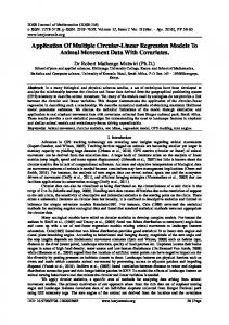
The methodology used in this paper is a modification of the technique done by Serbert et. al (1998). It is a well known fact that the least trimmed sum of squares (LTS) is a high breakdown estimator, where breakdown point is defined as the smallest fraction of unusual data that can render the estimator useless. From figure No.1, it can be seen that the LTS produces a better regression line compared to LS in the presence of outliers. Figure 1. Results of LS vs LTS

250

outliers 200

OLS fit with outliers 150

y

y = 7.8168x - 25.855

100

y=4.9613x-0.0930 LTS fit with outliers

50

0 0

5

10

x

15

20

25

The proposed method in this paper uses the standardized predicted and residual values from the least trimmed of squares (LTS) fit rather than the least squares (LS) fit used in the method by Serbert et. al (1998). The LTS regression was proposed by Rousseeuw and Leroy (1987). This method is similar to the least squares but instead of using all the squared residuals, it minimizes the sum of the h smallest squared residuals. The objective function is

19 – 22 March 2001

Orange, California, USA

381


h

Minimize βˆ ∑ (r 2 ) i:n i =1

and it is solved either by random resampling (Rousseeuw and Leroy, 1987), a genetic algorithm (Burns, 1992) which is used in S-Plus (Programming Package) or forward search (Woodruff and Rocke, 1994) . In this paper, the genetic algorithm (Burns, 1992) was used to solve the objective function of LTS. Putting h = (n/2) + [(p + 1)/2] , LTS reaches the maximal possible value for breakdown point. We assumed that the “clean” observations will form a linear relationship that is a horizontal chain-like cluster on the predicted and residual plot. Therefore to identify a clean base subset, the single linkage algorithm is used since this is the best technique for identifying an elongated clusters. Virtually all clustering procedures provide little information as to the number of clusters present in the data. Hierarchical methods routinely produce a series of solutions ranging from n clusters to a single cluster. So it is necessary to get a procedure that will tell us the number of clusters actually exist in the data set, that is the cluster tree needs to be “cut” at a certain height . Therefore the number of clusters depend on the height of the cut. When this procedure is applied to the results of hierarchical clustering methods, it is sometimes referred to as “stopping rule”. The stopping rule used in this paper is proposed by Mojena(1977). This rule resembles a onetailed confidence interval based on the n-1 heights (joining distances) of the cluster tree. The proposed methodology can be summarized as the following: 1. Standardize the predicted and residual values from least trimmed of squares (LTS) fit. 2. The Euclidean distance instead of Mahalanobis distance between pairs of the standardized predicted and residual values from step 1 is used as the similarity measure since it is well known that the predicted values and the residuals are not correlated to each other. It is assumed that the observations that are not outliers will generally have a linear relationship, that is from a clustering point of view, one is looking for a horizontal long chain-like cluster. This kind of cluster can be identified successfully by single linkage clustering algorithm. 3. Form clusters based on tree height (ch, a measure of closeness) using the Mojena’s stopping rule (ch = h + ks h where h is the average height of the tree and sh is the sample standard deviation of heights and k is a specified constant). Milligan and Cooper (1985) in a comprehensive study , conclude that the best overall performance is when k is set to 1.25. 4. The clean data set is the largest cluster formed which includes the median , while the other clusters are considered to be the potential outliers. To illustrate the proposed methodology, wood specific gravity data set from Draper and Smith (1966) is considered in this paper. A comparison between methods done by Serbert et. al (1998) ans the proposed method which is referred as method 1 is demonstrated in the next example. 3.

Example

A real data set from Draper and Smith (1966, p.227) which has 20 observations and 5 regressor variables is used. Modification to the data set is done by Rousseeuw and Leroy (1987) so that observations 4, 6, 8, and 19 are xy-space outlying ( as in Table No. 1)

382



Table 1. Sample data with 4 outliers Obs no 1 2 3 4 5 6 7 8 9 10 11 12 13 14 15 16 17 18 19 20

X1 0.573 0.651 0.606 0.437 0.547 0.444 0.489 0.413 0.536 0.685 0.664 0.703 0.653 0.586 0.534 0.523 0.58 0.448 0.417 0.528

X2 0.1059 0.1356 0.1273 0.1591 0.1135 0.1628 0.1231 0.1673 0.1182 0.1564 0.1588 0.1335 0.1395 0.1114 0.1143 0.132 0.1249 0.1028 0.1687 0.1057

X3 0.465 0.527 0.494 0.446 0.531 0.429 0.562 0.418 0.592 0.631 0.506 0.519 0.625 0.505 0.521 0.505 0.546 0.522 0.405 0.424

X4 0.538 0.545 0.521 0.423 0.519 0.411 0.455 0.43 0.464 0.564 0.481 0.484 0.519 0.565 0.57 0.612 0.608 0.534 0.415 0.566

X5 0.841 0.887 0.92 0.992 0.915 0.984 0.824 0.978 0.854 0.914 0.867 0.812 0.892 0.889 0.889 0.919 0.954 0.918 0.981 0.909

Y 0.534 0.535 0.57 0.45 0.548 0.431 0.481 0.423 0.475 0.486 0.554 0.519 0.492 0.517 0.502 0.508 0.52 0.506 0.401 0.568

In Table No. 2 are the standardized predicted and residuals values for the method by Serbert et. al (1998) and the proposed method (Method 1). Table 2. Results: Method 1 vs Serbert Serbert obs 1 2 3 4 5 6 7 8 9 10 11 12 13 14 15 16 17 18 19 20

Pred.values 1.1873 0.7728 0.9178 -1.4006 0.5368 -1.3900 -0.9846 -1.8146 -0.3869 -0.1174 0.1201 1.1026 0.0637 1.0916 0.3562 -0.1324 0.5914 -0.0434 -1.7371 1.2665

residuals -0.8447 0.0550 1.4478 0.4132 1.1678 -0.5264 1.0563 -0.0406 -0.4613 -0.4835 2.3135 -1.3953 -0.5656 -1.4693 -0.6834 0.6102 -0.2969 0.3307 -1.2625 0.6350

Proposed method (Method1) Pred. values -0.4427 -0.3458 0.3414 1.7183 -0.1368 1.8722 -1.0633 1.6732 -0.9235 -0.9851 0.0773 -0.4985 -0.9066 -0.4271 -0.7351 -0.6414 -0.4152 -0.3858 1.9284 0.2961

residuals 0.6249 0.5719 0.4804 -1.6401 0.5680 -1.9340 0.4896 -1.8857 0.3373 0.4896 0.4896 0.5085 0.4995 0.4414 0.4896 0.4896 0.4643 0.3025 -2.2762 0.4896

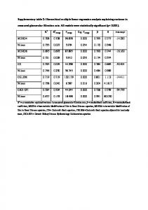
Below are the clusters ( Table No. 3) produced by Serbert’s method where the dendogram (Figure No. 2) is cut at the height of 0.9577 using the Mojenas’s stopping rule. There are three clusters formed and the cluster with the largest size which is cluster 1 is considered to contain the

19 – 22 March 2001


383


“clean” observations while cluster 2 and cluster 3 contain the potential outliers. The potential outliers are observations 4, 6, 7, 8, 11 and 19. Swamping effect is evident since clean observations 7 and 11 are flagged as outliers. Table 3. Clusters: Serbert’s method obs.

1

2 3

4

5

6

7

8

9

10

11

12

13

14

15

16

17

18

19

20

clust.

1

1 1

2

1

2

2

2

1

1

3

1

1

1

1

1

1

1

2

1

1.0

11

1.2

Figure 2. Dendogram for Serbert’s method

19

7 8

5

18

16

13

14

12

0.0

10

9

15

2 0.2

17

3

1

0.4

4

6

20

0.6

Height

0.8

0.96

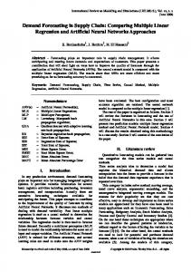
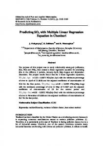
The following are the clusters ( Table No. 4) formed using the proposed method (method 1) where the dendogram (Figure No. 3) is cut at a height of 0.9656 based on Mojenas’s stopping rule. Two clusters are formed with cluster 2 being the cluster containing the “clean” observations while cluster 1 contains the potential outliers. This method correctly identifies all the outliers. Table 4. Clusters: Method 1 obs.

1

2 3

4 5

6

7 8

9

10

11

12

13

14

15

16

17

18

19

20

clust

2

2 2

1 2

1

2 1

2

2

2

2

2

2

2

2

2

2

1

2

It can be seen from the results obtained, method 1 is successful in flagging all the outliers. Although Serbert’s method is also successful in flagging all the outliers but it also wrongly flagged observations 7 and 11 as outliers. It is evident that the effect of swamping is present when Serbert’s method is used. A simulation study is conducted to test the performance of the proposed method (method 1)in various outlier scenarios and regression conditions. Since this methodology is a modification of Serbert’s method, it is logical that a comparison between these two methods are conducted using the scenarios proposed by Serbert et. al (1998).

384



0.97

4.

19 8

4

6

11 20

5 3

9 13

10

18

7

16

15

17

14

2

12

1

0.0

0.5

Height

1.0

1.5

2.0

2.5

Figure 3. Dendogram for method 1

Simulation study

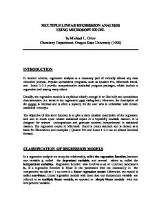
There are 6 outlier scenarios and a total of 24 different outlier situations ( each scenario consists of 4 situations differing in the percentage of outliers, distance from clean observations and the number of regressors) considered in this research . Figure No. 4 shows a simple regression picture of the six outlier scenarios chosen for this research. For each of the simulations, the value of the regression coefficients was set to be 5. The distribution of the regressor variables for the clean observations was set to be uniform U (0,20). The distribution of the error term for the clean and the outlying observations were assumed to be normal N(0,1). The following are the descriptions of the six scenarios. In scenario 1, there is one group of xyspace outlying observations with the regressor variable values approximately 20. There is one xyspace outlying group of outlying observations in scenario 2, but with the regressor variable values of approximately 30. While in scenario 3, there are two xy-space outlying groups where one group with regressor variable values of approximately 20 and the other group with regressor variable values of approximately 0. Scenario 4 is the same as scenario 3 except that in scenario 4, the regressor variable values are approximately –10 and 30. In the case of scenario 5, there is one x-space outlying group where the regressor variable values approximatly 30 . In the last scenario which is scenario 6, there is one x-space outlying group and one xy-space outlying group both with regressor variable values approximately 30. The factors considered in this simulation are similar to the “classic” data sets found in the literature. The levels for percentage of outliers are typically 10% and 20%. The number of outlying groups are one or two. The number of regressors is either 1, 3, or 6. The distances for the outliers were selected to be 5 standard deviations and 10 standard deviations. The simulation scenarios place a cluster or two clusters of several observations at a specified location shifted in X- space (outlying only in the regressor variables only), shifted in Y-space (outlying in the response variable only) and also shifted in XY-space The primary measures of performances are: (1) the probability that an outlying observation is detected (tppo) and (2) the probability that a known clean observation is identified as an outlier (tpswamp) that is, the occurrence of false alarm. Code development and simulations were done using S-Plus for Windows version 4.5 (Statistical Package).

19 – 22 March 2001


385


Figure 4. 6 Outliers scenario scen ario 2

scen ario 1

0

0

20

30

20

30

20

30

scen ario 4

scen ario 3

0

20

0

-1 0

scen ario 6

scen ario 5

0

4.1

20

20

30

0

Results of Simulations

1.2

tppo/tpswamp

1 0.8 0.6

Method1 Serbert

0.4

tpswamp, method1 tpswamp, Serbert's

0.2 0 1

2

3

4

5

6

7

8

9 10 11 12 13 14 15 16 17 18 19 20 21 22 23 24 Scenarios

Figure No. 5 : Comparison of performances between method1 and Serbert's for n = 20 and p = 1

386


IDENTIFYING MULTIPLE OUTLIERS IN LINEAR REGRESSION : ROBUST FIT AND CLUSTERING APPROACH 1.2

tppo/tpswamp

1 0.8 0.6 tppo,method1

0.4

tppo, Serbert tpswamp, method1

0.2

tpswamp, Serbert

0 1

2

3

4

5

6

7

8

9 10 11 12 13 14 15 16 17 18 19 20 21 22 23 24 Situations

Figure N o. 6 : Comparison of performance between method1 and Serbert's for n = 40 and p = 1

1.2

tppo/tpswamp

1 0.8 tppo, method 1

0.6

tppo, Serbert tpswamp, method 1

0.4

tpswamp, Serbert

0.2 0 1 2 3 4 5 6 7 8 9 10 11 12 13 14 15 16 17 18 19 20 21 22 23 24

Situations

Figure No. 7 : Comparison of performance for method 1 and Serbert's with n = 20 and p = 3

1.2

tppo/tpswamp

1 0.8 tppo, method1

0.6

tppo, Serbert tpswamp, method 1

0.4

tpswamp, Serbert

0.2 0 1 2 3 4 5 6 7 8 9 10 11 12 13 14 15 16 17 18 19 20 21 22 23 24 Situations

Figure No. 8 : Comparison of performance between method 1 and Serbert's for n = 40 and p = 3

Figure 5 shows that the detection probability (tppo) for the proposed method ( method 1) is better than Serbert’s in every scenarios except in situations 21 through 24 (scenario 6 in Figure No.4) where there are two outlying groups with one of them an x-space outlying observations and the other is an xy-space outlying observations.The probability of swamping (tpswamp) is also lower in method 1 compared to Serbert’s method , that is, lower probability of false alarm. But both methods have difficulty in detecting outliers in situations 3, 9, 11, 15, and 21 through 24. Figure 6 illustrates that the detection probability improves significantly for both methods when the sample size increases from n = 20 to n = 40, but method 1 still outperforms Serbert's in situations 3 and 11 where the percentage of outliers present is 20% and the distance of outliers from the clean data is 5 sigma.

19 – 22 March 2001


387


1.2

tppo/tpswamp

1 0.8 0.6

Serbert method1

0.4

tpswamp, method 1 tpswamp, Serbert's

0.2 0 1

2

3

4

5

6

7

8

9 10 11 12 13 14 15 16 17 18 19 20 21 22 23 24

Scenarios Figure No. 9 : Comparison of performances for method1 and Serbert's for n = 20 and p = 6

1.2

tppo/tpswamp

1 0.8

method1 Serbert

0.6

tpswamp, method1

0.4

tpswamp, Serbert's

0.2 0 1

2

3

4

5

6

7

8

9 10 11 12 13 14 15 16 17 18 19 20 21 22 23 24 scenarios

Figure No. 10 : Comparison of performances between method1 and Serbert's for n = 40 and p = 6

Figures 7 and 8 show that both methods performed much better at detecting outliers when the number of regressors increases from p = 1 to p = 3. For n = 20, both methods have difficulty in detecting outliers in situations 3 and 11 but method 1 still outperforms Serbert’s in those situations. As n increases from 20 to 40, both methods are equally good in every situations. Method 1 has a smaller probability of swamping in most of the situations. Figures 9 and 10 illustrate the performances of both methods when p = 6. The detection probability for method 1 is significantly lower than Serbert’s in situations 3, 11 and 12 when the sample size is 20 but improves when n is increased from 20 to 40. For n = 20, the probability of swamping is greater in method 1 than Serbert’s in situations 3, 7, 8, 11, 15, 16, 17, 19 and 20.

5.

Conclusions

Many authors have suggested using a clustering based approach in detecting multiple outliers. Among others, Gray and Ling (1984) propose a clustering algorithm to identify potentially influential subsets. Hadi and Simonoff (1993) propose a clustering strategy for identifying multiple outliers in linear regression by using the single linkage clustering on Z = [Xy]. As mentioned earlier, Serbert et. al (1998) also propose a clustering based method by using the single linkage clustering on the residual and associated predicted values from a least squares fit. The

388



proposed method, method 1 is a modification of Serbert’s, that is, replacing the least squares fit with a more robust fit which is the least trimmed of squares (LTS). From the simulation results obtained in section 3, method 1 is better than Serbert’s in detecting outliers in situations where the number of regressors p is less than or equal to 3 for small n (n = 20). The success of detecting outliers for method 1 can be improved significantly and as competitive as Serbert’s with the increase in the sample size even for situations where the number of regressors p is large. It is hoped that other clustering algorithm, may be a non hierarchical clustering algorithm, for example the kmeans clustering algorithm can be used effectively for identifying multiple outliers.

Reference Barnett, V. and Lewis, T. (1994), Outliers in Statistical Data, 3rd ed , John Wiley , Great Britain. Burns, P.J.(1992). “ A genetic algorithm for robust regression estimation,” StatSci Technical Note, Seattle, WA. Draper and Smith (1966), Applied Regression Analysis, New York, John Wiley and Sons, New York. Gray, J.B. and Ling, R.F., (1984), “K-clustering as a detection tool for influential subsets in regression, Technometrics 26, 305-330. Hadi, A. S. and Simonoff, J.S. (1993), “ Procedures for the Identification of Multiple Outliers in Linear Models”, Journal of the American Statistical Association, vol 88, No. 424. Hocking , R.R. (1996), Methods and Applications of Linear models - Regression and Analysis of Variance, John Wiley, New York. Mojena, R. (1977), “Hierarchical grouping methods and stopping rules: An evaluation”. The Computer Journal, 20, 359-363. Milligan G. W., and Cooper, M.C. (1985), “An Examination of Procedures for Determining the Number of Clusters in a Data Set”. Psychometrika, Vol. 50, No. 2, 159-179. Rousseeuw and Leroy (1987), Robust Regression and outlier detection, John Wiley & Sons, New York. Serbert, D.M., Montgomery,D.C. and Rollier, D. (1998). “A clustering algorithm for identifying multiple outliers in linear regression,” Computational Statistics & Data Analysis, 27, 461-484.

19 – 22 March 2001


389