0. Then by continuity (Assumption 1) and Lemma 3, ∂/∂θk Φ(θi ) > 0 for all i sufficiently large. Thus by Conditions 3 and 6,
so setting in θS i = θiS i in (38) and applying Condition 5 yields
(k) i (θ S (k) ; θi ) > 0 ∇10 k φ
i i i 2 i i+1 i i Ckθi+1 S i − θ S i k ≤ φ (θ S i ; θ ) − φ (θ S i ; θ ),
for all i ∈ Ik sufficiently large. But since φ(k) (·; θ i ) is strictly (k) i (θS (k) ; θi ) > 0, then θki+1 > concave (Condition 2), if ∇10 k φ i i θk . This contradicts θk → 0, so if θk∞ = 0 we must have ∂/∂θk Φ(θ ∞ ) ≤ 0, establishing the Karush-Kuhn-Tucker con2 ditions.
0
i i+1 (1 − t)Ji ((1 − t)θ i+1 S i + tθ S i ; θ ) dt (θ S i − θ S i ). (38)
From Condition 4, it follows that
where C = CS(θ 0 ) . We have used the fact that x0 Ax ≥ 2 kxk2 λmin {A} for any positive definite matrix A. kθi+1 − θi k → 0 as i → ∞.
Lemma 3
Proof: Since {Φ(θi )} is monotone increasing (Lemma 1) and bounded above (by continuity of Φ and compactness (Lemma 1) of S(θ 0 ), see p. 78 of [50]), it follows that Φ(θ i+1 ) − Φ(θ i ) → 2 0. Apply Lemma 2. Lemma 4 The sequence {θi } has a limit point4 θ? . For any such limit point, if θk? > 0, then ∂θ∂k Φ(θ ? ) = 0. Proof: By Lemma 1 and [50] (p. 56) there is a subsequence im and limit point θ ? ∈ S(θ 0 ) such that kθim −θ? k2 → 0 as m → ∞. Now pick any index k, and define km to be the smallest i ≥ im such that i ∈ Ik . By Condition 6, km ≤ im + imax . By the triangle inequality: kθkm − θ ? k2 ≤ kθkm − θim k2 + kθim − θ ? k2 ; the second term of which goes to 0 as m → ∞. For the first term, applying the triangle inequality repeatedly: kθkm − θim k2 ≤
iX m −1
kθi+1 − θi k2 ,
Since a strictly concave objective has only one point that satisfies the Karush-Kuhn-Tucker conditions, namely the constrained maximum, the limit θ∞ must be that point. Lemma 6 thus establishes global convergence under a generic set of assumptions and conditions. All that remains is to verify that the conditions are satisfied for the SAGE algorithms presented in this paper. Remark: In all of SAGE algorithms in this paper, the φi functionals are additively separable in their first argument, which means that the curvature matrices Ji (θS i ; θi ) are diagonal. In this case, Condition 5 reduces to verifying that the diagonal elements of Ji have a positive lower bound. This is clearly the case for convex penalties such as the quadratic penalty (30). In other words, for separable φi functionals, a sufficient condition for Condition 5 is: Condition 50 : For any bounded set S , there exists a CS > 0 such that for all θ ∈ S
i=km
which is a sum of at most imax terms by Condition 6, each of which goes to 0 as m → ∞ by Lemma 3. Thus kθkm −θ? k → 0 as m → ∞. Again using the triangle inequality: kθ
km +1
? 2
− θ k ≤ kθ
km +1
−θ
km 2
k + kθ
km
? 2
−θ k .
Thus kθkm +1 − θ? k → 0 as m → ∞. Since km ∈ S (k) , i.e. on iterations {km } one updates θk , (k) km (θS (k) ; θkm ) = 0. Taking the by Condition 4: θkkm +1 · ∇10 k φ limit as m → ∞ and using continuity (Condition 2) shows: (k) ? (θ S (k) ; θ? ) = 0. The Lemma then follows from θk? · ∇10 k φ 2 Condition 3. 4 The reader should note the distinction between limits and limit points (or cluster points) (p. 55 of [50]).
−
1 ∂ P (θ) ≥ CS . 2 ∂θk2
Theorem 1 A sequence {θi } generated by any of the PMLSAGE algorithms for penalized maximum-likelihood image reconstruction converges globally to the unique maximum of a strictly concave objective function Φ having a penalty function satisfying Condition 50 , provided zki > 0 ∀k. Proof: • Assumption 2 follows from the behavior of the Poisson log-likelihood as λk → ∞ [1]. • Condition 1 follows from Theorem 1 of [9].
11 • Condition 2 is easily verified for the hidden-data spaces and penalty functions used in this paper. • Condition 3 follows by the construction of φk using (5)(7). • Condition 4 is built into the definition (3), and is satisfied by (33).
probably be of limited academic interest since one rarely iterates a ML algorithm to convergence in the unregularized, underdetermined case. If one is willing to be content with a local convergence result, then it is possible to relax the assumption of strict concavity for the φi functionals, using a region of convergence idea similar to that in [9,13]. IX. ACKNOWLEDGEMENT
• Condition 5 follows from Condition 5’ since the SAGE algorithms have separable φi functionals. • Condition 6 is inherently satisfied by the cyclical sequential update used in PML-SAGE.
2
If one hopes for global convergence, then Condition 50 is a reasonable restriction; it is clearly satisfied for the quadratic penalty (30), and for most strictly convex penalties. There is an important technical difference between our proof and the assumptions in [1]. In [1] it was assumed that the sequence was initialized in the interior of Θ+ , and remained in the interior of Θ+ for every iteration. With our new complete-data spaces and hidden-data spaces, the iterates can come and go from boundary of Θ+ since the terms zki are nonzero. However, when zki is positive, one can verify that the corresponding functions φk are well-defined and differentiable on an open interval containing zero. Condition 2 as stated is only met if zki > 0 for all k, which will be true if rn > 0 for all n. If one were to include the effects of say, cosmic radiation, then in practice it is always the case that rn > 0. However, if some rn , and hence some zki are zero, it is simple to modify the proof to establish global convergence to the maximum. There is one important technical detail however; one cannot use zki > 0 in one iteration and then switch to zki = 0 in a later iteration, since then λik could get stuck on the boundary of Θ+ . Provided that one consistently uses either only the original complete-data space or only the new complete-data spaces, then global convergence is assured. As stated above, the proof does not always apply to the unpenalized maximum-likelihood algorithms ML-EM-1, ML-EM-3, and ML-SAGE-1,2,3 because the curvature assumption Condition 5 is not necessarily satisfied without a strictly convex penalty. However, one can replace Condition 5 with an alternative condition that each φi (θ S i ; θi ) must be a monotonically decreasing function of θk . This approach was used in [1,11]. With this condition, a small modification of the above proof establishes global convergence of the unpenalized algorithms, provided that Assumption 1 is still satisfied. This strict concavity will not be satisfied if the system matrix A does not have full column rank. We consider this to be a minor point since in the underdetermined case regularization is particularly essential, and the above proof shows that PML-SAGE converges globally for strictly concave penalized maximum-likelihood objectives. We conjecture that the methods of [53] could be extended to establish convergence of ML-EM-3, ML-SAGE-1,2,3, etc. without the strict concavity assumption, but such a proof would
The authors gratefully acknowledge Neal Clinthorne and W. Leslie Rogers for helpful discussions, Stephanie Sandor for bringing the mmap() function to their attention, and Ed Hoffman for providing the digital brain data. R EFERENCES [1] K Lange and R Carson, “EM reconstruction algorithms for emission and transmission tomography”, J. Comp. Assisted Tomo., vol. 8, no. 2, pp. 306–316, Apr. 1984. [2] S Joshi and M I Miller, “Maximum a posteriori estimation with good’s roughness for three-dimensional opticalsectioning microscopy”, J. Opt. Soc. Amer. Ser. A, vol. 10, no. 5, pp. 1078–1085, May 1993. [3] D L Snyder, A M Hammoud, and R L White, “Image recovery from data acquired with a charge-couple-device camera”, J. Opt. Soc. Amer. Ser. A, vol. 10, no. 5, pp. 1014–1023, May 1993. [4] A P Dempster, N M Laird, and D B Rubin, “Maximum likelihood from incomplete data via the EM algorithm”, J. Royal Stat. Soc. Ser. B, vol. 39, no. 1, pp. 1–38, 1977. [5] D G Politte and D L Snyder, “Corrections for accidental coincidences and attenuation in maximum-likelihood image reconstruction for positron-emission tomography”, IEEE Trans. Med. Im., vol. 10, no. 1, pp. 82–89, Mar. 1991. [6] M E Daube-Witherspoon, R E Carson, Y Yan, and T K Yap, “Scatter correction in maximum likelihood reconstruction of PET data”, in Conf. Rec. of the IEEE Nuc. Sci. Symp. Med. Im. Conf., 1992. [7] R Molina and B D Ripley, “Deconvolution in optical astronomy. A Bayesian approach”, in Stochastic Models, Statistical Methods, and Algorithms in Im. Analysis, P Barone, A Frigessi, and M Piccioni, Eds., vol. 74 of Lecture Notes in Statistics, pp. 233–239. Springer, New York, 1992. [8] J A Fessler and A O Hero, “Complete-data spaces and generalized EM algorithms”, in Proc. IEEE Conf. Acoust. Speech Sig. Proc., 1993, vol. 4, pp. 1–4. [9] J A Fessler and A O Hero, “Space-alternating generalized expectation-maximization algorithm”, IEEE Trans. Sig. Proc., vol. 42, no. 10, pp. 2664–2677, Oct. 1994.
12
REFERENCES
[10] J A Fessler, “Hidden data spaces for maximum-likelihood PET reconstruction”, in Conf. Rec. of the IEEE Nuc. Sci. Symp. Med. Im. Conf., 1992, vol. 2, pp. 898–900.
[23] X L Meng and D B Rubin, “Maximum likelihood estimation via the ECM algorithm: A general framework”, Biometrika, vol. 80, no. 2, pp. 267–278, 1993.
[11] J A Fessler, N H Clinthorne, and W Leslie Rogers, “On complete data spaces for PET reconstruction algorithms”, IEEE Trans. Nuc. Sci., vol. 40, no. 4, pp. 1055–1061, Aug. 1993.
[24] C H Liu and D B Rubin, “The ECME algorithm: a simple extension of EM and ECM with faster monotone convergence”, Biometrika, vol. 81, no. 4, 1994, To appear.
[12] J A Fessler and A O Hero, “New complete-data spaces and faster algorithms for penalized-likelihood emission tomography”, in Conf. Rec. of the IEEE Nuc. Sci. Symp. Med. Im. Conf., 1993, pp. 1897–1901. [13] A O Hero and J A Fessler, “Asymptotic convergence properties of EM-type algorithms”, Tech. Rep. 282, Comm. and Signal Proc. Lab., Dept. of EECS, Univ. of Michigan, Ann Arbor, MI, 48109, Apr. 1993. [14] A O Hero and J A Fessler, “Convergence in norm for alternating expectation-maximization (EM)-type algorithms”, Statistica Sinica, vol. 5, no. 1, pp. 0–0, Jan. 1995, To appear. [15] E Veklerov and J Llacer, “Stopping rule for the MLE algorithm based on statistical hypothesis testing”, IEEE Trans. Med. Im., vol. 6, no. 4, pp. 313–319, Dec. 1987. [16] J A Fessler, “Penalized weighted least-squares image reconstruction for positron emission tomography”, IEEE Trans. Med. Im., vol. 13, no. 2, pp. 290–300, June 1994. [17] K Lange, M Bahn, and R Little, “A theoretical study of some maximum likelihood algorithms for emission and transmission tomography”, IEEE Trans. Med. Im., vol. 6, no. 2, pp. 106–114, June 1987. [18] E M Levitan and G T Herman, “A maximum a posteriori probability expectation maximization algorithm for image reconstruction in emission tomography”, IEEE Trans. Med. Im., vol. 6, no. 3, pp. 185–192, Sept. 1987. [19] B W Silverman, M C Jones, J D Wilson, and D W Nychka, “A smoothed EM approach to indirect estimation problems, with particular reference to stereology and emission tomography”, J. Royal Stat. Soc. Ser. B, vol. 52, no. 2, pp. 271–324, 1990. [20] D L Snyder, M I Miller, L J Thomas, and D G Politte, “Noise and edge artifacts in maximum-likelihood reconstructions for emission tomography”, IEEE Trans. Med. Im., vol. 6, no. 3, pp. 228–238, Sept. 1987. [21] C S Butler and M I Miller, “Maximum A Posteriori estimation for SPECT using regularization techniques on massively parallel computers”, IEEE Trans. Med. Im., vol. 12, no. 1, pp. 84–89, Mar. 1993. [22] T Hebert and R Leahy, “A generalized EM algorithm for 3-D Bayesian reconstruction from Poisson data using Gibbs priors”, IEEE Trans. Med. Im., vol. 8, no. 2, pp. 194–202, June 1989.
[25] A R De Pierro, “A generalization of the EM algorithm for maximum likelihood estimates from incomplete data”, Tech. Rep. MIPG119, Med. Im. Proc. Group, Dept. of Radiol., Univ. of Pennsylvania, 1987. [26] A R De Pierro, “A modified expectation maximization algorithm for penalized likelihood estimation in emission tomography”, 1994, To appear in IEEE Trans. Med. Im. [27] M Abdalla and J W Kay, “Edge-preserving image restoration”, in Stochastic Models, Statistical Methods, and Algorithms in Im. Analysis, P Barone, A Frigessi, and M Piccioni, Eds., vol. 74 of Lecture Notes in Statistics, pp. 1–13. Springer, New York, 1992. [28] S Geman and D E McClure, “Bayesian image analysis: an application to single photon emission tomography”, in Proc. of Stat. Comp. Sect. of Amer. Stat. Assoc., 1985, pp. 12–18. [29] S Geman and D E McClure, “Statistical methods for tomographic image reconstruction”, Proc. 46 Sect. ISI, Bull. ISI, vol. 52, pp. 5–21, 1987. [30] P J Green, “Bayesian reconstructions from emission tomography data using a modified EM algorithm”, IEEE Trans. Med. Im., vol. 9, no. 1, pp. 84–93, Mar. 1990. [31] P J Green, “Statistical methods for spatial image analysis (discussion)”, Proc. 46 Sect. ISI, Bull. ISI, vol. 52, pp. 43–44, 1987. [32] K Lange, “Convergence of EM image reconstruction algorithms with Gibbs smoothing”, IEEE Trans. Med. Im., vol. 9, no. 4, pp. 439–446, Dec. 1990, Corrections, June 1991. [33] Z Liang, R Jaszczak, and K Greer, “On Bayesian image reconstruction from projections: uniform and nonuniform a priori source information”, IEEE Trans. Med. Im., vol. 8, no. 3, pp. 227–235, Sept. 1989. [34] G T Herman and D Odhner, “Performance evaluation of an iterative image reconstruction algorithm for positronemission tomography”, IEEE Trans. Med. Im., vol. 10, no. 3, pp. 336–346, Sept. 1991. [35] G T Herman, D Odhner, K D Toennies, and S A Zenios, “A parallelized algorithm for image reconstruction from noisy projections”, in Large-Scale Numerical Optimization, T F Coleman and Y Li, Eds., pp. 3–21. SIAM, Philadelphia, 1990.
REFERENCES [36] A W McCarthy and M I Miller, “Maximum likelihood SPECT in clinical computation times using meshconnected parallel processors”, IEEE Trans. Med. Im., vol. 10, no. 3, pp. 426–436, Sept. 1991. [37] M I Miller and B Roysam, “Bayesian image reconstruction for emission tomography incoporating Good’s roughness prior on massively parallel processors”, Proc. Natl. Acad. Sci., vol. 88, pp. 3223–3227, Apr. 1991. [38] A D Lantermann, “A new way to regularize maximumlikelihood estimates for emission tomography with Good’s roughness penalty”, Tech. Rep. ESSRL-92-05, Elec. Sys. and Sig. Res. Lab., Washington Univ., Jan. 1992. [39] D L Snyder, A D Lanterman, and M I Miller, “Regularizing images in emission tomography via an extension of Good’s roughness measure”, Tech. Rep. ESSRL-92-17, Washington Univ., Jan. 1992. [40] C Bouman and K Sauer, “Fast numerical methods for emission and transmission tomographic reconstruction”, in Proc. 27th Conf. Info. Sci. Sys., Johns Hopkins, 1993, pp. 611–616. [41] C Bouman and K Sauer, “A unified approach to statistical tomography using coordinate descent optimization”, 1993, Submitted to Trans. Im. Proc. [42] E U Mumcuoglu, R Leahy, S R Cherry, and Z Zhou, “Fast gradient-based methods for Bayesian reconstruction of transmission and emission PET images”, Tech. Rep. 241, Signal and Image Processing Inst., USC, Sept. 1993. [43] J A Fessler and A O Hero, “Space-alternating generalized EM algorithms for penalized maximum-likelihood image reconstruction”, Tech. Rep. 286, Comm. and Sign. Proc. Lab., Dept. of EECS, Univ. of Michigan, Ann Arbor, MI, 48109-2122, Feb. 1994. [44] A R De Pierro, “On the relation between the ISRA and the EM algorithm for positron emission tomography”, IEEE Trans. Med. Im., vol. 12, no. 2, pp. 328–333, June 1993. [45] L Kaufman, “Implementing and accelerating the EM algorithm for positron emission tomography”, IEEE Trans. Med. Im., vol. 6, no. 1, pp. 37–51, Mar. 1987. [46] A O Hero and J A Fessler, “A recursive algorithm for computing Cramer-Rao-type bounds on estimator covariance”, IEEE Trans. Info. Theory, vol. 40, no. 4, pp. 1205–1210, July 1994. [47] K Sauer and C Bouman, “A local update strategy for iterative reconstruction from projections”, IEEE Trans. Sig. Proc., vol. 41, no. 2, pp. 534–548, Feb. 1993. [48] W H Press, B P Flannery, S A Teukolsky, and W T Vetterling, Numerical Recipes in C, Cambridge Univ. Press, 1988.
13 [49] H M Hudson and R S Larkin, “Acceleration image reconstruction using ordered subsets of projection data”, IEEE Trans. Med. Im., vol. 0, no. 0, pp. 0–0, 0 1994, To appear. [50] M Rosenlicht, Introduction to Analysis, Dover, New York, 1985. [51] R E Williamson, R H Crowell, and H F Trotter, Calculus of Vector Functions, Prentice Hall, New Jersey, 1972. [52] A M Ostrowski, Solution of equations in Euclidian and Banach spaces, Academic Press, 1973. [53] T M Cover, “An algorithm for maximizing expected log investment return”, IEEE Trans. Info. Theory, vol. 30, no. 2, pp. 369–373, Mar. 1984.
REFERENCES
14
Type-I Algorithm (e.g. ML-EM, PML-OSL) and Type-II Algorithm (e.g. PML-GEM) Initialize λ0 for i = 0, 1, . . . { y¯n
=
sn
=
ek
=
X
ank λik + rn , n = 1, . . . , N
k
yn /¯ yn , n = 1, . . . , N X ank sn , k = 1, . . . , p
(39) (40)
n
for k = 1, . . . , p { = gk (ek ; λi ), λi+1 k
λi+1 k }
?
i
= gk (ek ; λ ; λ ),
(Type-I) (see (14), (21), (22), (23), (37))
(41)
or (Type-II) (see (36))
(42)
}
Initialize λ0 , for i = 0, 1, . . . {
Type-III Algorithm (e.g. ML-SAGE, PML-SAGE) P y¯n = k ank λ0k + rn , n = 1, . . . , N . k
=
ek
=
1 + (i modulo p) X ank yn /¯ yn
(43)
n
λi+1 k λi+1 j y¯n
=
gk (ek ; λi ) (see (27), (33))
=
λij ,
(44)
j 6= k,
:= y¯n + (λi+1 − λik )ank , ∀n : ank 6= 0 k
(45)
} Table 1: Three generic pseudo-code algorithm types for penalized maximum-likelihood image reconstruction. All of the algorithms presented in the text are of one of these three types. Within each type, the algorithms differ in form of the functions g() used in the M-step.
REFERENCES
15
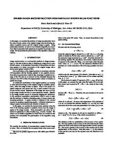
Figure 1: Digital brain phantom (left), and filtered backprojection reconstructed image (right).
16
REFERENCES
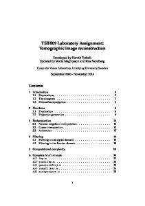
Figure 2: PML-SAGE-2 estimates from data with 5% random coincidences at iterations i = 0, 5, 10, 20 (left to right). Top row: initialized with uniform image. Middle row: initialized with thresholded filtered-backprojection image. Bottom row: absolute value of difference between top and middle rows amplified by a factor of 4.
REFERENCES
17
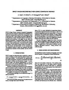
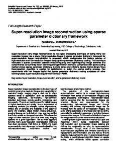
Penalized Maximum Likelihood - Quadratic Penalty 6000
Penalized Log-Likelihood
5500 5000 4500 4000
PML-SAGE-3 PML-LINU-1 PML-GEM-1,3
3500
PML-SAGE-1,2 PML-OSL-1,3
3000 2500 2000 0
0% Randoms 5
10
15
20 Iteration
25
30
35
40
Figure 3: Penalized likelihood Φ(λi ) − Φ(λ0 ) vs. iteration from data with 0% random coincidences.
REFERENCES
18
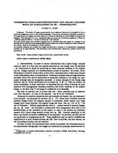
Penalized Maximum Likelihood - Quadratic Penalty
Penalized Log-Likelihood
3000
2500
2000 -
PML-SAGE-3 PML-LINB-1
1500
PML-GEM-3 PML-GEM-1
1000
PML-OSL-1 500 5% Randoms 0 0
5
10
15
20 Iteration
25
30
35
40
Figure 4: Penalized likelihood Φ(λi ) − Φ(λ0 ) vs. iteration from data with 5% random coincidences. Not shown is PML-SAGE-2, which converges slightly slower than PML-SAGE-3. Also not shown is PML-SAGE-1, which is indistinguishable from PMLOSL-1.
REFERENCES
19
Penalized Maximum Likelihood - Quadratic Penalty 1400
Penalized Log-Likelihood
1200 1000 -
800
PML-SAGE-2 PML-LINB-1 PML-GEM-3
600
PML-GEM-1 PML-OSL-1
400 200 35% Randoms 0 0
5
10
15
20 Iteration
25
30
Figure 5: As in Fig. 3, but with 35% random coincidences.
35
40