As a solution to this degeneracy problem, we show that the penalization ... Inverse Wishart prior on covariance matrices eliminates the degeneracies in this case ...
arXiv:physics/0111007v1 [physics.data-an] 2 Nov 2001
Penalized maximum likelihood for multivariate Gaussian mixture Hichem Snoussi∗ and Ali Mohammad-Djafari∗ ∗
Laboratoire des Signaux et Systèmes (L2S), Supélec, Plateau de Moulon, 91192 Gif-sur-Yvette Cedex, France Abstract. In this paper, we first consider the parameter estimation of a multivariate random process distribution using multivariate Gaussian mixture law. The labels of the mixture are allowed to have a general probability law which gives the possibility to modelize a temporal structure of the process under study. We generalize the case of univariate Gaussian mixture in [1] to show that the likelihood is unbounded and goes to infinity when one of the covariance matrices approaches the boundary of singularity of the non negative definite matrices set. We characterize the parameter set of these singularities. As a solution to this degeneracy problem, we show that the penalization of the likelihood by an Inverse Wishart prior on covariance matrices results to a penalized or maximum a posteriori criterion which is bounded. Then, the existence of positive definite matrices optimizing this criterion can be guaranteed. We also show that with a modified EM procedure or with a Bayesian sampling scheme, we can constrain covariance matrices to belong to a particular subclass of covariance matrices. Finally, we study degeneracies in the source separation problem where the characterization of parameter singularity set is more complex. We show, however, that Inverse Wishart prior on covariance matrices eliminates the degeneracies in this case too.
INTRODUCTION We consider a double stochastic process: A discrete process (zt )t=1..T , with zt taking its values in the discrete set Z = {1..K}. • A continuous process (st )t=1..T which is white conditionally to the first process (zt )t=1..T and following a distribution:
•
p(s|z) = f (s; ζz ) In the following, without loss of generality of the considered model, we restrict the function f (.) to be a Gaussian: f (.|z) = N (µz , Rz ). This double process is called in literature "Mixture model". When the hidden process P z1..T is white, we have an i.i.d mixture model: p(s) = z pz N (µz , Rz ) and when z1..T is Markovian, the model is called HMM (Hidden Markov Model). For application of these two models see [2] and [3]. Mixture models present an interesting alternative to non parametric modeling. By increasing the number of mixture components, we are able to approximate any probability density and the time dependence structure of the hidden process z1..T allows to take into account a correlation structure of the resulting process. In the following, for clarity of demonstrations, we assume an i.i.d. mixture model.
CHARACTERIZATION OF LIKELIHOOD DEGENERACY We consider T observations (st )t=1..T of a random n-vector following a multivariate Gaussian mixture law: p(st ) =
K X
pz N (st ; µz , Rz )
z=1
Where pz = P (Z = z) is the probability that the random hidden label Z takes the value z ∈ Z = {1..K}, µz is the n-vector mean of the Gaussian component z and Rz its n × n covariance matrix. We intend to estimate the parameters θ z = (pz , µz , Rz )z∈1..K by maximizing its likelihood given the observations s1..T = [st ]t=1..T : b = arg max p(s1..T | θ) θ θ∈Θ
Where p(s1..T | θ) =
T X Y t=1
z
pz |2πRz |
(−1/2)
�
1 exp − (st − µz )T R−1 z (st − µz ) 2
�
and o n P n p = 1; R ∈ R; µ ∈ R Θ = θ z = (pz , µz , Rz ) | pz ∈ R+ , K z z z=1 z
(1)
R is a closed subset of covariance matrices. Some examples of R are considered later in section 4 and in [4]. Proposition 1 [Likelihood function is unbounded]: ∀ s1..T ∈ (Rn )T , ∃ a singularity point θ s in the parameter space Θ such that: lim p(s1..T | θ) = ∞. These points are the θ→θs
θ = (pz , µz , Rz )z∈Z such that, at least one of the Rz (but not all of them together) is a singular non negative matrix and the correspondent mean µz lies in the intersection of n − rank(Rz ) hyperplans of Rn . Proof: Let z0 ∈ Z and Rz0 be a singular NND matrix of rank p < n. Rz0 can be diagonalized in the orthogonal group: 0 .. . 0 T Rz0 = U ΛU , Λ= λ n−p+1 .. . λn
� � (n) Consider now a sequence of positive definite matrices Rz0
n∈N
(n) T Rz 0 = U
(n)
λ1
..
. (n)
λn−p λn−p+1 ..
. λn
�
(n) λi
defined by:
�
U
With the (n − p) strictly positive numeric sequences which tend to 0. i=1..(n−p) � � (n) Thus the sequence of Rz0 converges to Rz0 . Likelihood function evaluated at n∈N
(n)
Rz0 is:
pn (s1..T | θ) =
T � Y
(−1/2) pz0 |2πR(n) exp z0 |
t=1
X + pz N (µz , Rz ) z
!
�
1 −1 − (st − µz0 )T R(n) (st − µz0 ) z0 2
�
Expending the exponent of the component z0 in canonical form : −1
(st − µz ) = (st − µz )T R(n) z0
X [U (st − µ )]2 z i (n)
i
(n)
λi
,
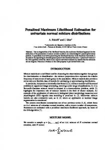
We can see that when the eigenvalues (λi )i=1..(n−p) tend to zero, or equivalently, when (n) the covariance Rz0 tends to Rz0 and when µz0 lies in the intersection of the hyperplans (Hi = {µ | [U (st − µ)]i = 0})i=1..(n−p), the likelihood function goes to infinity. So we have proved that any singular NND matrix is a point of degeneracy provided that the means lie in specific hyperplans. In one dimensional case, this corresponds to the fact that σ goes to zero and the correspondent mean coincides with one observation. Figure 1 shows an example of this degeneracy. In this example, we take an original distribution of a 2-D random vector which is a mixture of 10 Gaussians. The Gaussians have their means located on a cercle and have the same covariance. Figure 1-a shows the graph of this distribution from which we generated 100 samples in order to estimate its parameters. Figure 1-b shows the estimated distribution. We can note the failure of the maximum likelihood estimator and its tendency to converge to sharp Gaussians. Here, we highlight the effect of growing the dimension n which increases the occurrence of degeneracy. We have, for n > 1 an infinite number of singularities. Moreover, even if we fix the means of the mixture components, the unboundedness of likelihood might occur if some covariances go to particular singular matrices . But, we think that this second kind of degeneracy is less likely to happen particularly if the number of
samples grows. We note that the occurrence of degeneracy increases when the dimension grows and decreases when the number of samples grows.
0.04
0.08
0.035
0.07
0.03
0.06
0.025
0.05
0.02
0.04
0.015
0.03
0.01
0.02
0.005
0.01
0 5
0 5 5
5
0
0 0 −5
0 −5
−5
Original distribution
−5
ML Estimated distribution with 100 samples
Fig-1. Failure of the ML estimation of the parameters of a 10 component Gaussian mixture distribution.
BAYESIAN SOLUTION TO DEGENERACY This degeneracy was noted by many authors (Day, 1969 [5]) and in (Hathaway 1986 [6]), a constraint formulation of the EM algorithm has been proposed to eliminate this degeneracy. In (Ormoneit 1998 [7]), a penalization by an Inverse Wishart prior was employed to eliminate it. Our contribution leads to the same penalization but in different manner. In (Ormoneit 1998), the Inverse Wishart prior was chosen because it is a conjugate prior. In the one dimensional case [1], the penalization by an Inverse Gamma prior on variances was used to eliminate degeneracy. In this work, after characterizing the origin of these singularities, we extend this procedure to the multivariate case to propose an Inverse Wishart prior on covariances Rz which guarantees the boundness of the likelihood: pα,β,J (Rz ) =
� �� K −1 exp −α Tr R J z |Rz |β
where K is a normalization constant, α and β two strictly positive constants which contain a priori information about the power level (scale parameter) and J is a positive definite symmetric matrix which contains a priori information on the covariance structure. In fact, the mode of this law is given by: ∂ log [p(Rz )] −1 −1 = −βR−1 z + αRz J Rz = 0 ∂Rz Leading to: Rz =
α J β
Proposition 2: ∀ s1..T ∈ (Rn )T , the a posteriori distribution p(θ | s1..T ) with the a priori: Y p(θ) = pαz ,βz ,Jz (Rz ) z∈Z
is bounded and goes to 0 when one of the covariance matrices Rz approaches a singular matrix. Proof: The penalized likelihood is: p(s1..T | θ) p(θ) =
T Y t=1
(
Y
p(Rz ))1/T
X
pz N (µz , Rz )
z
z∈Z
!
For each label z, we have the following inequality: (
Y
p(Rz ))1/T N (µz , Rz ) ≤
z∈Z
� �� A Y Kz exp −αz Tr Rz −1 Jz 1/2 β z |Rz | z∈Z |Rz |
Thus, to prove the proposition, we need to show that ∀ a > 0, b > 0 and Rs a singular matrix, we have: � �� 1 exp −a Tr R−1 =0 z J b Rz −→Rs |Rz | lim
Using the inequality
(det A)1/n ≤
1 Tr (A) n
valid for any real symmetric n × n matrix A, We have: � � � �� 1 |J |1/n 1 −1 exp −a Tr Rz J ≤ exp −a n |Rz |b |Rz |b |Rz |1/n
In the above inequality, the right hand side term goes to zero when Rz approaches the boundary of singularity. Therefore, the penalized likelihood is bounded and is null on the boundary of singularity. At this point, we can also follow the arguments in [4] to prove the existence of positive definite matrices corrresponding to the modes of the penalized likelihood. Figure 2 illustrates the regularization effect of this penalization. Here we used the same samples
generated for the figure 1 and estimated the parameters of the mixture by optimizing the penalized likelihood criterion. The probability of degeneracy is zero.
0.04
0.06
0.035 0.03 0.04
0.025 0.02 0.015
0.02
0.01 0.005 0 5
0 5 5
5
0
0 0 −5
0 −5
−5
Original distribution
−5
Penalized EM Estimated distribution with 100 samples
Fig-2. Regularization effect of the penalized EM algorithm.
ESTIMATION OF STRUCTURED COVARIANCE MATRICES In this paragraph, we generalize the work in [4] to estimate covariance matrices of specified structure in the mixture case. The constraints are summarized in the closed subset R introduced in the definition of the parameter set Θ (1).
Unconstrained case: The unconstrained case was treated in many works. In [7], three methods were proposed: Averaging, maximum penalized likelihood and Bayesian sampling. We briefly recall the EM algorithm and the Bayesian sampling which both can be seen as data augmentation algorithms: •
EM algorithm: It consists of two steps: (i) E (Expectation)-step: Consider observations s1..T as incomplete data and (s1..T , z1..T ) as complete data and compute the functional Q(θ | θ (k) ) = E{log p(s1..T , z1..T | θ) + log p(θ) | s1..T , θ (k) }; (ii) M (Maximization)-step: Update θ (k+1) = arg maxθ Q(θ | θ (k) ).
•
Bayesian sampling: It consists of two steps: (k+1) (i) Generate z1..T ∼ p(z1..T | s1..T , θ (k) ); (k+1) (ii) Generate θ k+1 ∼ p(θ | s1..T , z1..T ).
In the unconstrained case, one obtains, in both first steps of the above algorithms, functionals which have only one maximum obtained by canceling the gradient to zero.
Constrained case: In both EM algorithm and Bayesian sampling methods presented above, the second step which consists in updating θ was unconstrained. We see in the following how we are able to combine the data augmentation algorithms with the iterative gradient algorithm proposed in [4] to constrain the covariance matrix Rz to be in the closed set R.
Strutured EM The functional Q(θ | θ(k) ) can be decomposed as follows: Q(θ | θ
(k)
)=
K X
g(Rz , Sz ) + f (p, µ | θ (k) )
z=1
with: (
� � αJ (S + ) g(Rz , Sz ) = −(1 + Nβz ) log |Rz | − Tr R−1 z z Nz PT (k) Nz = t=1 p(z(t) = z | s(t), θ )
and Sz the weighted sample covariance matrix: Sz =
PT
(k+1) (k+1) ∗ ) (s(t) − µz ) p(z(t) t=1 (s(t) − µz PT (k) ) t=1 p(z(t) = z | s(t), θ
= z | s(t), θ (k) )
Thus, the maximization of Q with respect to Rz is equivalent to the maximization of g(Rz , Sz ) with respect to Rz . The necessary gradient equations are: � � β α J −1 −1 −1 )Rz − (1 + )R )δRz = 0 (2) δg(Rz , Sz ) = Tr (Rz (Sz + Nz Nz z In the unconstrained case, the solution of (2) is Rz =
J Sz + α N z
1+ Nβ
. Constraint maximization
z
of g with Rz ∈ R for any R is not easy. However, if R is such that R ∈ R ⇒ δR ∈ R (for example the set of Toeplitz matrices) then we replace the second step of the EM algorithm by the following: (k+1)
(k)
(k+1)
1. Find Dz belonging to R so that g(Rz , Sz − Dz gradient conditions. (k+1) (k) (k+1) 2. Put Rz = Rz + Dz
) satisfies the necessary
This modification preserves the monotonicity of the EM algorithm and makes the problem linear in Dz and so it is easier to impose constraints with the condition that the variation of Rz still belongs to R, which is true for a wide range of constraints such in the Toeplitz case.
Structured Bayesian sampling We propose the following Bayesian sampling scheme: ∗ 1. Generate z1..T ∼ p(z1..T | s1..T , θ (k) ); (k+1)
2. Generate Dz belonging to R accordingi to the a posteriori distribution h (k) (k+1) ∗ p(Dz | s1..T , z1..T ) ∼ exp g(Rz , Sz − Dz ) . (k+1)
3. Update Rz
(k)
(k+1)
= Rz + Dz
∗ Sz is the sample covariance depending on the partition defined by z1..T : ( P s(t)s(t)∗ z Sz = t∈T Card(Tz ) Tz = {t | z(t) = z}
To be sure that the sampling keeps Dz in the closed set R, we define a basis (Ql )l=1..L ∗ of R and we sample the projection of Dz on R: x1..L ∼ p(x1..L | s1..T , z1..T ), where the vector x1..L is defined as: Dz =
L X
xl Ql
l=1
MIXED SOURCES We consider now the case where sources are not directly observed, but mixed with an unknown mixing matrix A and we want to take into account measurement errors so that observations are modeled by the following equation: x(t) = A s(t) + n(t) In this section, we show that when we are interested in estimating jointly the mixing matrix A, noise covariance matrix Rǫ and the parameters of the mixture, by maximizing the likelihood p(x1..T | A, Rǫ , θ z ), we encounter the same problems of degeneracy mentioned above. Likelihood function has the following expression: p(x1..T | A, Rǫ , θ z ) =
T X K Y
pz (t)N (Aµz , ARz A∗ + Rǫ )
t=1 z=1
with θ z = (µz , Rz , pz ). The expression pz (t) =
X
p(z1..T ) represents the marginal law of z(t). Indeed,
z1..T ,z(t)=z
the hidden variables do not need necessarily to be white and so the mixture to be i.i.d. We can rewrite the expression of the likelihood in a more general form in which the
marginalization is not performed : p(x1..T | A, Rǫ , θ z ) =
X
z1..T
p(z1..T )
T Y
N (Aµz , ARz A∗ + Rǫ )
t=1
It is obvious, under this form, that degeneracy happens when one of the terms constituting the sum tends to infinity and this is independently of the law p(z1..T ). Consider now the matrices Γz = ARz A∗ + Rǫ . It’s clear that degeneracy is produced when, among matrices Γz , at least one is singular and one is regular. We show in the following that this situation can occur. We recall that the matrices Rz and Rǫ belong to a closed subset of the set of the non negative definite matrices. Constraining matrices to be positive definite leads to complicated solutions. The main origin of this complication is the fact that the set of positive definite matrices is not closed. For the same reason, we don’t constrain the mixing matrix A to be of full rank. Proposition 3: ∀ A non null, ∃ matrices {Γz = ARz A∗ + Rǫ for z = 1..K} such that {z | Γz is singular} = 6 ∅ and {z | Γz is regular} = 6 ∅. Rǫ is necessarily a singular NND matrix and Card ({z | Rz is regular}) < K.
Proof: Without affecting the generality of the problem, we show how to construct a singular matrix Γ1 and the others matrices Γz regular. We consider NND matrices. Therefore, the kernel of the correspondent linear mapping coincides with its isotropic cone. Thus, we have: Ker(Γz ) = Ker(ARz A∗ ) ∩ Ker(Rǫ ) It is sufficient to prove the existence of Rǫ and (Rz )z=1..K that verify the following condition: � Ker(AR1 A∗ ) ∩ Ker(Rǫ ) 6= {0} (3) Ker(ARz A∗ ) ∩ Ker(Rǫ ) = {0} , z = 2..K If the matrix Rǫ is regular, there is no degeneracy: According to the mini-max principle applied to the characterization of the eigenvalues of the sum of two hermitian matrices, the eigenvalues of Γz are greater than those of Rǫ and then strictly positive which imply that all of the matrices Γz are regular. We have: Ker(A∗ ) ⊆ Ker(ARz A∗ ), z = 1..K
(4)
Equality holds if Rz is regular or if Ker(Rz ) ∩ Im(A∗ ) = {0}. Note that if all the matrices Rz are regular, there is no degeneracy. Suppose then that the matrices Rz , except the first matrix R1 , are regular. We will try now to construct the matrices R1 and Rǫ making the condition (3) verified. Let a
non null vector xs belong to [Ker(A∗ )]⊥ . There exist NND matrices R1 and Rǫ such that xs ∈ Ker(AR1 A∗ ) ∩ Ker(Rǫ ). In fact, consider the family of vectors (xj )j∈J belonging to Ker(A∗ ) such that the family {xs } ∪ (xj )j∈J is orthogonal (this is insured P by the principle of the incomplete basis). The matrices R1 = j∈J αj xj x∗j (αj ≥ 0) P and Rǫ = j∈J βj xj x∗j (βj ≥ 0) are such that xs ∈ Ker(AR1 A∗ ) ∩ Ker(Rǫ ) by construction and Ker(ARz A∗ ) ∩ Ker(Rǫ ) = {0}. We have then constructed matrices which verify the degeneracy condition. Note that the fact that the matrices R1 and Rǫ are singular is a necessary condition but not sufficient; the matrix R1 can be singular with Ker(AR1 A∗ ) = Ker(A∗ ) and so there is no degeneracy, or as well, Rǫ is singular but Ker(ARz A∗ ) ∩ Ker(Rǫ ) 6= {0}, ∀z ∈ {1..K}, which implies that all matrices Γz are singular and so no degeneracy occurs.
DEGENERACY ELIMINATION IN THE MIXED CASE In the light of what we presented in the two first paragraphs, one possible way to eliminate this degeneracy consists in penalizing the likelihood by an Inverse Wishart a priori for covariance matrices. In fact, we know that the origin of degeneracy is that the covariance matrices Rz and Rǫ approach the boundary of singularity (in a non arbitrary way). Thus, if we penalize the likelihood such that when one of the covariance matrices approaches the boundary, the a posteriori distribution goes to zero, eliminating the infinity value at the boundary and even forcing it to zero. Proposition 5: ∀ x1..T ∈ (Rm )T , the likelihood p(x1..T | θ z , Rǫ , A) penalized by an a priori Inverse Wishart for the noise covariance matrix Rǫ or by an a priori Inverse Wishart for the matrices Rz is bounded and goes to 0 when one of the covariance matrices approaches the boundary of singularity.
Proof 5: The proof is based upon the proof of the proposition 4, except the fact that here the a priori is not directly related to the matrices Γz = ARz A∗ + Rǫ , but to covariance matrices Rz or Rǫ . Then, we have the following alternative: •
If one penalizes by an a priori Inverse Wishart on the matrix Rǫ , we have the following inequality: (p(Rǫ ))1/T N (Aµz , Γz ) ≤
� �� K A −1 exp −α Tr R J ǫ |Γz |1/2 |Rǫ |β
Now according to the mini-max principle applied to the characterization of eigenvalues, we have: |Γz | = |ARz A∗ + Rǫ | ≥ |Rǫ |
which yields the following inequality: (p(Rǫ ))1/T N (Aµz , Γz ) ≤
� �� 1 −1 exp −a Tr R J ǫ |Rǫ |b
This insures the convergence to 0 of the penalized likelihood when Rǫ goes to a singular matrix and insures, as well, the elimination of degeneracy which one the necessary conditions is the singularity of the covariance Rǫ . • If we penalize only by an Inverse Wishart prior on the matrices Rz with an uniform a priori on the matrix Rǫ , we have a similar inequality: (p(Rz ))1/T N (Aµz , Γz ) ≤
� �� 1 −1 exp −a trace R J z z z |ARz A∗ |bz
Here, the only query is that the determinant |A| goes to zero faster than the exponential of |Rz | but, in this situation, the degeneracy condition (3) is not verified because of the inclusion relation (4).
CONCLUSION The set of parameter singularities which characterizes the likelihood degeneracy of a multivariate Gaussian mixture is identified. A Bayesian solution to this degeneracy is proposed. We proposed a modified version of the data augmentation algorithms which allows to account for some constraints on the structure of the covariance matrices of the Gaussian mixture distribution. It consists essentially in the introduction of an inverse iteration to make the problem linear with respect to the matrix estimate. The case of source separation with Gaussian mixture model sources is also considered and discussed.
REFERENCES 1. A. Ridolfi and J. Idier, “Penalized maximum likelihood estimation for univariate normal mixture distributions”, in Actes du 17e colloque GRETSI, Vannes, September 1999, pp. 259–262. 2. H. Snoussi and A. Mohammad-Djafari, “Bayesian source separation with mixture of gaussians prior for sources and gaussian prior for mixture coefficients”, in Bayesian Inference and Maximum Entropy Methods, A. Mohammad-Djafari, Ed., Gif-sur-Yvette, July 2000, MaxEnt Workshops, to appear in. 3. H. Snoussi and A. Mohammad-Djafari, “Bayesian separation of HMM sources”, in Bayesian Inference and Maximum Entropy Methods. MaxEnt Workshops, August 2001, to appear in. 4. J. P. Burg, “Estimation of structured covariance matrices”, Proceeding of ieee, vol. 70, no. 9, pp. 963–974, September 1982. 5. N. Day, “Estimating the components of a mixture of normal distributions”, Biometrika, vol. 56, pp. 463–474, 1969. 6. R. J. Hathaway, “A constrained EM algorithm for univariate normal mixtures”, J. Statist. Comput. Simul., vol. 23, pp. 211–230, 1986. 7. D. Ormoneit and V. Tresp, “Averaging, maximum penalized likelihood and Bayesian estimation for improving Gaussian mixture probability density estimates”, IEEE Transactions on Neural Networks, vol. 9, no. 4, pp. 639–649, July 1998.