Multiresolution Histograms and their Use for Texture ... - Columbia CS

Multiresolution Histograms and their Use for Texture Classification E. Hadjidemetriou, M. D. Grossberg, and S. K. Nayar Computer Science, Columbia University, New York, NY 10027 {stathis, mdog, nayar}@cs.columbia.edu Abstract

Bin Count

Gaussian Filtering

2 Prior Work Two approaches to incorporate texture information into the histogram is to compute the histograms of image blocks [3], or the set of locally orderless histograms [7]. These ap-

400 200

64

128

192

255

128

192

255

Intensity

4000 3000 2000 1000 0 0

64

Intensity 12500

Bin Count

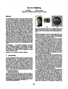
1 The Multiresolution Histogram The histogram of image intensities has proven to be a robust and efficient representation for indexing visual databases [15]. Histograms, however, don’t encode texture information. The multiresolution decomposition of an image does encode texture information. The histograms of Gaussian blurred versions of an image, as shown in Fig. 1, encode the interactions between intensities of neighboring parts of the image. We call this sequence of histograms the multiresolution histogram. This representation retains many important properties of the histogram. It is fast to compute, space efficient, and invariant to rigid motions. The inherent blurring also makes it robust to noise. All these properties make this an effective texture feature. In this work we make the following contributions: (1) We present a simple yet novel texture feature based on the multiresolution histogram. (2) We evaluate the performance of our feature. It gives excellent results on two texture databases while maintaining considerable robustness to illumination. (3) We compare our feature with five of the most commonly used texture features. We show that our simple feature is comparable or better in terms of discriminability, robustness, and efficiency.

600

0 0

Bin Count

The histogram of image intensities is used extensively for the retrieval of images from visual databases. An obvious way to extend this feature is to compute the histograms of multiple resolutions of an image. Both this extension and the plain histogram are fast to compute, space efficient, invariant to rigid motions, and robust to noise. In addition, the histograms over multiple image resolutions directly encode texture information. We describe a simple yet novel matching algorithm based on this extension. We evaluate it on two texture databases against algorithms based on five widely used texture features. We show that with our simple algorithm, we achieve or exceed the performance, robustness, and efficiency of more complicated features.

Multiresolution Histogram

10000 7500 5000 2500

Original Image

0 0

64

128

192

Intensity

255

Figure 1. The left column shows the original image and two images resulting from blurring with a Gaussian filter. The right column shows the multiresolution histogram, which is the sequence of histograms of the filtered images. proaches do not directly provide a single global feature encoding texture. Texture features have been obtained by taking the histogram of the output of a derivative filter applied to the image. Two filters that have been used are differences of Gaussians [16], and Gabor filters [6]. Derivative filters have been preferred because there has been a general belief that Gaussian filtering introduces an erroneous bias [16]. Derivative filtering, however, is notoriously sensitive to noise. Also, the sensitivity of derivative filtering to texel and texture parameters has only been examined to a very limited extent. The histogram of lower resolutions of an image suffers from the same inability to encode texture as that suffered by the histogram of the original image [13]. Heeger [9] used histograms of multiple resolutions of an image sequentially for texture synthesis. Hadjidemetriou et al performed a sensitivity analysis of the multiresolution histogram with respect to parameters of synthetic texels and textures [8]. This analysis

J1

demonstrated that the multiresolution histogram is a robust texture representation.

5 4

3 Properties of Multiresolution Histograms

3

The multiresolution histogram is a family of histograms hτ for different image resolutions τ . We obtain the multiresolution histogram from an image L by convolving the image with a Gaussian filter1 G(τ ), followed by taking the histogram to obtain h τ (L) = h(L ∗ G(τ )), for several τ . The multiresolution histogram is invariant to translation, rotation, and is robust to noise. We make the multiresolution histogram robust to changes in illumination by equalizing the histogram of the initial image. To examine analytically the sensitivity of the multiresolution histogram we consider a weighted average of incremental changes of histogram bin counts with respect to the image resolution τ , which gives the Fisher information measure, J: J(L) =

2 m−1


σ 2

(−vj ln vj )

j=0

dhj (L ∗ G(τ )) , dτ

(a) Shape Elongation: ρ

filter is defined G(τ ) =

2 −y 2 1 exp −x , 2πτ σ 2 2τ σ 2

with the st. dev. σ.

2

3

4

5

(b)

x 10 5

J1 6

ρ

4 3

(c) Shape Boundary: η

2

0

2

J1 0.08

(d)

4

6

η

6

p

0.06 0.04 0.02 0

(e) Texel Number: p

1

2

3

4

5

(f)

J1 0.029

(1)

where x = (x, y) is a point in the domain D of the image [17]. In images that contain parameterized texels or textures the Fisher information measure becomes a function of these parameters. The dependence of the Fisher information on some of these parameters has been examined [8]. A simple parameter of a texel is its elongation. The elongation is a linear stretching ρ of one of the axes while contracting the other axis by 1/ρ. Elongating an image preserves its histogram. Fig. 2 (a) shows one image from a family of elongated images. A strongly elongated texel blurs faster with respect to resolution. A plot of the Fisher information vs. elongation shown in Fig. 2 (b) confirms this. It can be shown that the Fisher information satisfies J ∝ (ρ + 1/ρ) [8]. The multiresolution histogram is also sensitive to the complexity of the texel boundary. When a boundary of a texel has a sharp corner it blurs more rapidly than when it is smooth. This is confirmed for a family of parametric superquadric texels, normalized to have the same area and thus histogram. Three instances of this family are shown in Fig. 2 (c) with η the family’s parameter. A plot of the Fisher information as a function of this parameter is shown in Fig. 2 (d). The plot shows that the change in the histogram with image resolution is minimized for a circle, η = 2. A simple texture parameter is the number of texels. The Fisher information is proportional to this parameter [8]. Fig. 2 (e) shows images of textures with p×p texels, for three

2 1

5

0.028 0.027 0.026

where vj is the intensity value of bin j [8]. The Fisher information can also be written in terms of the image gradient:     ∇L(x) 2 2   J(L) = (2)  L(x)  L(x)d x, D

1 The

6

Ordered

Random

(g) Texel Placement: σP

0.025 0

5

10

15

(h)

20

σP

Figure 2. Examples of the Fisher information as a function of texel and texture parameters. values of p. The histogram is independent of the number of texels. The plot in Fig. 2 (f) shows that the multiresolution histogram is sensitive to this parameter. Another texture parameter is the randomness of the placement of the texels [19]. The left image in Fig. 2(g) shows a texture whose texels are placed at regular intervals. As we move to the right, the placement of the texels in the image is perturbed using Gaussian noise with increasing standard deviation, σP . The histogram of the image is not significantly affected. Fig. 2 (h) shows a plot of the Fisher information as a function of σ P . Increasing the standard deviation of this perturbation decreases monotonically the change of the histogram with image resolution. This shows, along with the examples above, that the multiresolution histogram is sensitive to both texel and texture parameters.

4

Matching Algorithm

The properties we have described make the multiresolution histogram a good basis for a texture feature. The steps of the algorithm are shown in Fig. 3. (1) We implement the Burt-Adelson image pyramid [2]. It involves Gaussian smoothing sufficient for a pyramid subsampling factor of four. (2) We compute the histograms. (3) The histograms of each level of the pyramid are smoothed and normalized to have unit L 1 norm. (4) We then compute the cumulative histograms. This makes the feature more robust to noise. (5) Next we compute the differences between cumulative histograms of consecutive levels. This makes the feature inde-

Construct Image Pyramid

(2)

Compute Histograms

(3) (4)

Compute Feature

(1)

Compute Cumulative Histograms

(5)

Compute Differences

(6)

Subsample and Normalize

(7)

Compare using L1 norm

Figure 3. The steps of our matching algorithm. pendent of the original histogram. (6) To improve the matching, the difference histograms are subsampled and normalized to make them independent of the subsampling factor. The results are concatenated to form a feature vector. (7) Finally, the distance between two feature vectors is given by the L1 norm. The L 1 norm is commonly used with image histograms and statistical distributions [5, 13]. The performance depends on the choice of the histogram bin widths in step (6) of our algorithm. The bin width which gives the best performance depends mainly on the number of pixels and on the standard deviations of the histograms [5]. If there are l levels in the pyramid, then let S be the ˆl−1 be the standard pyramid subsampling factor, and σ ˆ 0, . . . σ deviations of the histograms for each level. It can be shown that the optimal bin widths w 0 , . . . , wl−1 have ratios given by σi+1 /ˆ σi ), wi+1 /wi = (S 1/3 )(ˆ

into several image classes. Each class contains different instances of the same texture. We tested using both constant bin widths, as well as bin widths chosen adaptively using Eq. (3). We used a single estimate of the standard deviations σ ˆ i for each database. We tried two subsampling factors in the experiments, the maximum possible, S 1/3 = 22/3 ≈ 1.59, and 21/2 ≈ 1.41. The subsampling factors were combined with an initial intensity resolution of 256 bins. Matching with noise was implemented by superimposing zero-mean Gaussian noise to a test image from the database. In a correct match the closest match to the test image was another database image of the same class. The first database consists of 13 Brodatz textures [1]. Each texture is scanned under seven rotation angles. The images are 179 × 179 pixels. Some of the database textures are shown in Fig. 4. Fig. 5 shows plots of the percentage of correct matches vs. the standard deviation of Gaussian noise. One of the plots in Fig. 5 was obtained with constant bin width of 8 bit/pixel and the other two plots were obtained with the two subsampling factors. The matching without noise is perfect since the multiresolution histogram is invariant to rotations. The matching is robust under noise. The highest histogram subsampling had the highest performance. Thus, the adaptive bin width improves performance, in addition to reducing cost. The second database is a random subset of the CUReT database [4] consisting of 61 physical textures under 131 or 132 instances of each physical texture under different illumination and viewing conditions. The total number of images is 8,046. The image size was 100 × 100 pixels. Some of the database textures are shown in Fig. 6. The percentages of correct matches as a function of Gaussian noise are shown in Fig. 7. To compute the matching percentage for a specific level of noise 100 images were ran-

(3)

where S is the ratio of image sizes between consecutive pyramid levels [5]. Thus, we can adaptively determine the bin widths2 for subsampling given the image pyramid. Prior to subsampling, the histograms are smoothed with a Gaussian to prevent aliasing. The cost of computing the multiresolution histograms is dominated by the cost of computing the Burt–Adelson pyramid. The latter cost is of order O(nr), where n is the number of pixels, and r is the width of the separable Gaussian filter.

Bark

Brick

Bubbles

Grass

5 Matching Performance

Leather

Pigskin

Raffia

Sand

We evaluated the matching performance of the algorithm given in Fig. 3 using two databases: a database of 91 Brodatz textures [1], and a database of 8,046 CUReT textures [4]. Both databases consist of 8-bit images of natural textures which we histogram equalized. Each databases is divided

Straw

Weave

Wood

Wool

2 If the sequence σ ˆ0 , . . . σ ˆl−1 decreases monotonically, σ ˆi+1 /ˆ σi ≤ 1, then the ratio of bin widths is bounded above by S1/3 .

Figure 4. Samples from the database of Brodatz textures [1]. All the images are histogram equalized.

Class without orig. (%)

95 90 85 80 75 70 65 60 0

Constant Bin Width Adaptive Bin Width Subsampling Factor=2 2/3 Subsampling Factor=2 1/2 10

20

30

40

50

60

Effect. st. dev. of noise (σ n)

ture vector consists of the L 2 norms of images resulting from the wavelets packets transform [12]. (4) Auto–cooccurrence matrices: The matrices are computed over a square window around a pixel of size 11 × 11 pixels. The feature is the entire matrix [10]. (5) Markov random field parameters: Each pixel is assumed to be a linear combination of the intensities in a 3 × 3 window surrounding it [14]. The parameters are computed with minimum norm least squares. The distance between all feature vectors was computed with the L1 norm, except the wavelet packets features whose distance was computed with L 2 as described in the literature [12]. The only features invariant to rotation are the multiresolution histograms.

7 Figure 5. Plots of the percentage of correct matches using our algorithm vs. the standard deviation of Gaussian noise for the Brodatz textures database [1].

Figure 6. Samples from the database of CUReT textures [4]. All the images are histogram equalized.

domly selected from the database and used as test images. The matching rates in Fig. 7 were obtained with either constant or adaptive bin widths. The plots for adaptive bin width performed as well as and even better than those with constant bin width. The high matching performance of the multiresolution histograms for this database demonstrates the robustness of our matching algorithm to database size, number of database classes, and changes in illumination. It also demonstrates the algorithm is robust to image noise.

6 Texture Features used for Comparison We compare the multiresolution histogram against five other commonly used features. These features were: (1) Fourier power spectrum annuli: The Fourier power spectrum is segmented into annuli of constant thickness. The feature vector consists of the sum of the values over the different annuli [18]. (2) Gabor wavelet features: The components of the feature vector are the L 1 norms of the band–pass images [11]. (3) Daubechies wavelet packets features: The fea-

Evaluation of Features and Discussion

The experimental setup and the databases were described in the previous section. To make the comparison meaningful the best performing parameters were selected for each feature and for each database. The parameters for our algorithm were the same for both databases. We used an adaptive bin width with a subsampling factor of 2 1/2 ≈ 1.41. We first evaluated all the algorithms on the database of Brodatz textures. The plots of the matching rates as a function of noise are shown in Fig. 8 (a). The matching rate without noise in Fig. 8 (a) is an indication of the sensitivity to rotations. The noise free matching rate of the multiresolution histograms and Fourier power spectrum features is 100%. The performance of the remaining features is lower. Our second evaluation compared all the algorithms on the CUReT database. Fig. 8 (b) shows the percentage of correct matches vs. standard deviation of noise. We achieved the best results in the noise free case with the multiresolution histograms, the wavelet packets features, and the Gabor features. These features are robust with respect to database size and number of database classes. The remaining features are sensitive to these parameters. The two databases demonstrated our algorithm to be the most robust to image noise, image rotation, changes in illumination, and database size.

100

Class without orig. (%)

100

90 80 70 60 50 0

256, Constant Bin Width 128, Constant Bin Width 2/3 256, Subsampling Factor =2 256, Subsampling Factor =2 1/2

10

20

30

40

50

Effect. st. dev. of noise (σn )

Figure 7. Plots of the percentage of correct matches using our algorithm vs. the standard deviation of Gaussian noise for the CUReT textures database [4].

(a)

Class without orig. (%)

100

be very useful to apply our algorithm over a limited image region.

80

References

60 40 20 0

0

10

20

30

40

Effect. st. dev. of noise (σn)

50

60

Multiresolution diff. histograms Fourier power spectrum Gabor features Wavelet Packets Cooccurrence matrix Markov random fields

(b)

Class without orig. (%)

100 80 60 40 20 0

0

10

20

30

40

50

Effect. st. dev. of noise (σn) Multiresolution diff. histograms Fourier power spectrum Gabor features Wavelet Packets Cooccurrence matrix Markov random fields

Figure 8. The percentage of correct matches vs. noise added to a test image for each algorithm applied to the Brodatz database [1] in (a) and the CUReT database [4] in (b).

The most expensive feature to compute are the Markov random field parameters, since they involve the computation of a least squares pseudoinverse. The Gabor features become the most expensive to compute for large images. The cost of the Fourier power spectrum feature follows. Both the cost of auto-cooccurence matrices, and the cost of the wavelet features is moderate. The least expensive feature to compute is the multiresolution histogram, since it is computed over an image pyramid. Many common texture features involve derivative filtering or the use of a template. Such features are intuitive but very sensitive. The multiresolution histograms implicitly incorporates a derivative as the integrand of Eq. (2) shows. The same equations, however, also shows that our feature involves spatial integration which increases its robustness. This work could be extended to further determine the types of textures that have similar multiresolution histograms. Also, it would

[1] P. Brodatz. Textures: A Photographic Album for Artists and Designers. Dover Publications, New York, 1966. [2] P. Burt and E. Adelson. The Laplacian pyramid as a compact image code. IEEE Trans. on Comm., 31(4):532–540, 1983. [3] M. Carlotto. Texture classification based on hypothesis testing approach. In Proc. of IJCPR, pages 93–96, 1984. [4] K. Dana, S. Nayar, B. van Ginneken, and J. Koenderink. Reflectance and texture of real-world surfaces. In Proc. of CVPR, pages 151–157, 1997. [5] L. Devroye and L. Gyorfi. Nonparametric Density Estimation: The L1 View. John Wiley and Sons, Canada, 1985. [6] F. Farrokhnia and A. Jain. A multi-channel filtering approach to texture segmentation. In Proc. of CVPR, pages 364–370, 1991. [7] L. Griffin. Scale–imprecision space. Image and Vision Computing, 15:369–398, 1997. [8] E. Hadjidemetriou, M. Grossberg, and S. Nayar. Spatial information in multiresolution histograms. In Proc. of CVPR, 2001. [9] D. Heeger and J. Bergen. Pyramid–based texture analysis/synthesis. In Proc. SIGGRAPH, pages 229–234, 1995. [10] J. Huang, S. Kumar, M. Mitra, W. Zhu, and R. Zabih. Image indexing using color correlograms. In Proc. of CVPR, pages 762–768, 1997. [11] A. Jain, N. Ratha, and S. Lakshmanan. Object detection using Gabor filters. Pattern Recognition, 30(2):295–309, 1997. [12] A. Laine and J. Fan. Texture classification by wavelet packet signatures. IEEE Trans. on PAMI, 15(11):1186–1191, 1993. [13] J. Lee and B. W.Dickinson. Multiresolution video indexing for subband coded video databases. In Proc. of SPIE, volume 2185, pages 162–173, 1994. [14] J. Mao and A. Jain. Texture classification and segmentation using multiresolution simultaneous autoregressive models. Pattern Recognition, 25(2):173–188, 1992. [15] W. Niblack. The QBIC project: Querying images by content using color, texture, and shape. In Proc. of SPIE, volume 1908, pages 173–187, 1993. [16] S. Ravela and R. Manmatha. Retrieving images by appearance. In Proc. of ICCV, pages 608–613, 1998. [17] A. Stam. Some inequalities satisfied by the quantities of information of Fisher and Shannon. Information and Control, 2:101–112, 1959. [18] J. Weszka, C. Dryer, and A. Rosenfeld. A comparative study of texture measures for terrain classification. IEEE Trans. on Systems, Man, and Cybernetics, SMC-6(4):269–285, 1976. [19] J. Wijk. Spot noise-texture synthesis for data visualization. In Proc. of SIGGRAPH, pages 309–318, 1991.