Multiresolution Homogenization Schemes for Differential ... - CiteSeerX

Multiresolution Homogenization Schemes for Differential Equations and Applications Anna C. Gilbert

A Dissertation Presented to the Faculty of Princeton University in Candidacy for the Degree of Doctor of Philosophy

Recommended for Acceptance By the Department of Mathematics

June 1997

c Copyright by Anna C. Gilbert, 1997. All Rights Reserved

Abstract The multiresolution analysis (MRA) strategy for homogenization consists of two algorithms; a procedure for extracting the eective equation for the average or for the coarse scale behavior of the solution to a dierential equation (the reduction process) and a method for building a simpler equation whose solution has the same coarse behavior as the solution to a more complex equation (the homogenization process). We present two multiresolution reduction methods for nonlinear dierential equations; a numerical procedure and an analytic method. We discuss the convergence of the analytic method. We apply the MRA reduction methods to nd and to characterize the averages of the steady-states of a model reaction-diusion problem. We also compare the MRA methods for linear dierential equations to the classical homogenization methods for elliptic equations.

iii

Acknowledgements First, I would like to thank my advisor Ingrid Daubechies for her patience, guidance, and inspiration. She has been an excellent mentor both mathematically and personally. I would also like to thank Greg Beylkin and Mary Brewster. Their work set the stage for this thesis and we worked together on a major part of it. My visits to Paci c Northwest National Laboratories to work with Mary were very rewarding and enjoyable. I also thank Ioannis Kevrekidis for his interest and enthusiasm in this work. The nal portion of this thesis was completed through his encouragement. I have received nancial support and guidance through two dierent programs and two dierent companies. I thank Lawrence Cowsar and Wim Sweldens of Lucent Technologies for their support through the Ph.D. Fellowship program. I thank Robert Calderbank for his support at AT&T Labs (formerly AT&T Bell Laboratories) through the Graduate Research Program for Women. I would also like to thank my friends and colleagues in the mathematics, applied mathematics, and chemical engineering departments at Princeton University; especially George Donovan, Mark Johnson, Peter Kramer, Jonathan Mattingly, Stas Shvartsman, and Terence Tao for their many helpful discussions. I give personal thanks to my mother Lynn Gilbert for her support and encouragement. I also thank my father and stepmother John and Vicki Gilbert for their support. I give thanks to Phyllis and Walter Strauss for welcoming me into their family. Finally, I would like to thank Martin Strauss for his love and patience.

iv

To my family.

v

Contents Abstract . . . . . . Acknowledgements List of Tables . . . List of Figures . . .

. . . .

. . . .

. . . .

. . . .

. . . .

. . . .

. . . .

. . . .

. . . .

. . . .

. . . .

. . . .

. . . .

. . . .

. . . .

. . . .

. . . .

. . . .

. . . .

. . . .

. . . .

. . . .

. . . .

. . . .

. . . .

. . . .

. . . .

. . . .

. . . .

. iii . iv . viii . ix

1 Introduction 2 A Comparison of MRA and Classical Homogenization Methods

1 5

2.1 Multiresolution Homogenization Method . . . . . . . . . . . . . 2.1.1 Reduction of Linear ODEs . . . . . . . . . . . . . . . . . 2.1.2 Augmentation Procedure for Linear ODEs . . . . . . . . 2.2 Second-order Elliptic Problems . . . . . . . . . . . . . . . . . . 2.2.1 Reduction Procedure without Forcing Terms . . . . . . . 2.2.2 Homogenization via Augmentation . . . . . . . . . . . . 2.2.3 Reduction Procedure with Forcing Terms . . . . . . . . . 2.3 Several approaches in classical homogenization theory: a review 2.3.1 Asymptotic Method . . . . . . . . . . . . . . . . . . . . 2.3.2 Flows . . . . . . . . . . . . . . . . . . . . . . . . . . . . 2.4 Physical Examples . . . . . . . . . . . . . . . . . . . . . . . . . 2.5 Conclusions . . . . . . . . . . . . . . . . . . . . . . . . . . . . .

3 MRA Reduction Methods for Nonlinear ODEs

3.1 Nonlinear Reduction Method . . . . . . . . . . . . . . 3.2 Series Expansion of the Recurrence Relations . . . . . . 3.2.1 Recursion Relations for Autonomous Equations 3.2.2 Algorithm to Generate Recurrence Relations . . 3.3 Convergence of the Series Expansion . . . . . . . . . . 3.3.1 Closed Form Expressions . . . . . . . . . . . . . 3.3.2 Convergence of the Lowest Two Order Terms . 3.3.3 Linear ODEs and Convergence Issues . . . . . . 3.4 Implementation and Examples . . . . . . . . . . . . . . 3.4.1 Implementation of the Reduction Procedure . . 3.4.2 Examples . . . . . . . . . . . . . . . . . . . . . vi

. . . . . . . . . . .

. . . . . . . . . . .

. . . . . . . . . . .

. . . . . . . . . . .

. . . . . . . . . . .

. . . .

. . . . . . . . . . . .

. . . . . . . . . . . .

. . . . . . . . . . . .

. . . . . . . . . . .

. . . . . . . . . . .

. . . . . . . . . . .

6 6 12 14 15 22 23 25 26 27 29 34

35 36 43 46 49 51 52 53 58 63 63 64

3.5 Homogenization . . . . . . . . . . . . . . . . . . . . . . . . . . . . . . 3.6 Conclusions . . . . . . . . . . . . . . . . . . . . . . . . . . . . . . . .

4 Steady-states of a model reaction-diusion problem

4.1 Setting the stage . . . . . . . . . . . . . . . . . . . . . 4.2 New Techniques . . . . . . . . . . . . . . . . . . . . . . 4.2.1 Recurrence relations for n-dimensional systems . 4.2.2 Boundary value problems . . . . . . . . . . . . 4.2.3 Rescaling the interval [0; 1] . . . . . . . . . . . . 4.2.4 Generalized Haar Basis . . . . . . . . . . . . . . 4.3 Characterizing the average in terms of L . . . . . . . . 4.4 Complexity of reduction algorithm . . . . . . . . . . . 4.5 Conclusions . . . . . . . . . . . . . . . . . . . . . . . .

5 Conclusions 6 Appendix A

. . . . . . . . .

. . . . . . . . .

. . . . . . . . .

. . . . . . . . .

. . . . . . . . .

. . . . . . . . .

. . . . . . . . .

. . . . . . . . .

74 75

77 79 80 81 82 83 87 89 96 96

98 99

vii

List of Tables 3.1 Errors as a function of the initial resolution . . . . . . . . . . . . . . 3.2 Error as a function of the number of sample points in s, with linear interpolation and with cubic interpolation . . . . . . . . . . . . . . . 3.3 Errors as a function of the intermediate resolution . . . . . . . . . . . 3.4 The entry xe is the value of x(t) for the corresponding initial value x0 , which we call a separation point. The ratio tells us if the separation point is stable or unstable. These three columns are calculated using the eective equation. We also calculate the separation point closest to x0 = 0 with an asymptotic method and a linear method. The rst error is the error between the asymptotic method and the reduction method and the second error is between the linear and the reduction methods. . . . . . . . . . . . . . . . . . . . . . . . . . . . . . . . . . . 4.1 This table lists the values of the coecients clm for the initial resolution level n = 15. . . . . . . . . . . . . . . . . . . . . . . . . . . . . . . . . 4.2 This table lists the averages of the solution u(x) over the interval [0; L] as a function of the interval length L. . . . . . . . . . . . . . . . . . .

viii

65 65 67

73 92 93

List of Figures 2.1 This gure shows the dierence between the fourth partial sum of (3 wavelets and the weight function in the Haar basis, P;4?1)1 biorthogonal k=0 4;k (t) ? (t). . . . . . . . . . . . . . . . . . . . . . . . . . . . . 2.2 This gure shows a comparison of the dierence between the MRA homogenized solution and the true solution Tnh(x) ? x (in the dotted line
) on one hand, and of the dierence between the asymptotic solution and the true solution T2? (x) ? x (in the dashed line -). Here n = 3 and  = 1. Both of the functions Tnh and T2? correspond to the temperature in a rod with period cells of length 2?n. . . . . . . . . . 2.3 This is a plot of the thermal conductivity (1x) = 2 ? sin(2 tan( 2 x)). This function \contains" a continuum of scales. . . . . . . . . . . . . 3.1 Maple code to compute recurrence relations for coecients up to any speci ed order in series expansions of g and f . The speci ed order for the example is ord := 2. The variable h stands for the  used in the text. . . . . . . . . . . . . . . . . . . . . . . . . . . . . . . . . . . . . 3.2 The error as a function of the number of sample points in s for linear and cubic interpolation methods . . . . . . . . . . . . . . . . . . . . . 3.3 The error as a function of the intermediate resolution level at which we switch from the analytic reduction method to the numerical reduction method. . . . . . . . . . . . . . . . . . . . . . . . . . . . . . . . . . . 3.4 The ows for equation (3.45) with zero forcing. . . . . . . . . . . . . 3.5 The ows for equation (3.45) with small but nonzero forcing. Notice that there are three periodic orbits, two stable and one unstable. . . . 3.6 The ows for equation (3.45) with large amplitude A. Notice that there is only one (stable) periodic orbit in this diagram as the system has undergone a pitchfork bifurcation. . . . . . . . . . . . . . . . . . . . . 4.1 This is a graph of 256 samples of the parameters a0 and a1 with base values ?0:4 and 2=3 (respectively) and defect values 0:65 and 4=3 (respectively). . . . . . . . . . . . . . . . . . . . . . . . . . . . . . . . .

22

n

n

ix

33 34

49 66 67 68 69 70 78

4.2 This is a graph of the average of the solution u(x) over the interval [0; L] as a function of the interval length L. Notice that there is an (almost) linear relationship between the average u0 and the period length L. . 4.3 This is a graph of the solution u(x) for period length L = 48:0. Because the solution u(x) is computed by the pseudo-spectral method there are small oscillations in the solution which are a result of Gibbs' phenomenon. . . . . . . . . . . . . . . . . . . . . . . . . . . . . . . .

x

94 95

Chapter 1 Introduction There are many important physical problems which incorporate multiple scales. The interactions and the neness of these scales make solving these problems on the nest scales prohibitively expensive. Often, we would be content with the coarse scale behavior of the solution but the ne scales aect this behavior so we cannot simply ignore these. Instead, it is useful to nd a way of extracting or constructing equations for the coarse behavior of the solution which take into account the eect of the ne scales. This amounts to writing an eective equation for the coarse scale component of the solution which can be solved much more economically. Alternatively, we might want to construct simpler ne scale equations whose solutions have the same coarse properties as the solutions of more complicated systems. These simpler equations would also be considerably less expensive to solve. These procedures are generally referred to as homogenization, though the speci cs of the approaches vary signi cantly. An example of a problem which encompasses many scales and which is dicult to solve on the nest scale is molecular dynamics. The highest frequency motion of a polymer chain under the fully coupled set of Newton's equations determines the largest stable integration time step for the system. In the context of long time dynamics the high frequency motions of the system are not of interest but current numerical methods (see [1],[22]) which directly access the low frequency motions of the polymer are ad hoc methods, not methods which take into account the eects of the high frequency behavior. The work of Bornemann and Schutte (see [19],[8]) is a notable exception and appears quite promising. Let us brie y mention several classical approaches to homogenization. The classical theory of homogenization, developed in part by Bensoussan, Lions, and Papanicolaou [4]; Jikov, Kozlov, and Oleinik [15]; Murat [18]; and Tartar[24], poses the problem as follows: Given a family of dierential operators L, indexed by a parameter , assume that the boundary value problem Lu = f in

(with u subject to the appropriate boundary conditions) is well-posed in a Sobolev 1

space H for all  and that the solutions u form a bounded subset of H so that there is a weak limit u0 in H of the solutions u. The small parameter  might represent the relative magnitude of the ne and coarse scales. The problem of homogenization is to nd the dierential equation that u0 satis es and to construct the corresponding dierential operator. We call the homogenized operator L0 and the equation L0 u0 = f in the homogenized equation. There are several methods for solving this problem. A standard technique is to expand the solution in powers of , to substitute the asymptotic series into the dierential equations and associated boundary conditions, and then to recursively solve for the coecients of the series given the rst order approximation to the solution (see [17], [3], and [16] for more details). If we consider a probabilistic interpretation of the solutions to elliptic or parabolic PDEs as averages of functionals of the trajectory of a diusion process, then homogenization involves the weak limits of probability measures de ned by a stochastic process ([4]). In [15] and [4], the methods of asymptotic expansions and of G-convergence are used to examine families of operators L. Murat and Tartar (see [18] and [24]) developed the method of compensated compactness. Coifman et al (see [12]) have recently shown that there are intrinsic links between compensated compactness theory and the tools of classical harmonic analysis (such as Hardy spaces and operator estimates). Using a multiresolution approach, Beylkin and Brewster in [9] give a procedure for constructing an equation directly for the coarse scale component of the solution. This process is called reduction. From this eective equation one can determine a simpler equation for the original function with the same coarse scale behavior. Unlike the asymptotic approach for traditional homogenization, the reduction procedure in [9] consists of a reduction operator which takes an equation at one scale and constructs the eective equation at an adjacent scale (the next coarsest scale). This reduction operator can be used recursively provided that the form of the equation is preserved under the transition. For systems of linear ordinary dierential equations a step of the multiresolution reduction procedure consists of changing the coordinate system to split variables into averages and dierences (in fact, quite literally in the case of the Haar basis), expressing the dierences in terms of the averages, and eliminating the dierences from the equations. For systems of linear ODEs there are relatively simple explicit expressions for the coecients of the resulting reduced system. Because the system is organized so that the form of the equations is preserved, we may apply the reduction step recursively to obtain the reduced system over several scales. Beylkin and Coult in [7] present a multiresolution approach to the reduction of elliptic PDEs and eigenvalue problems. They show that by choosing an appropriate MRA for a given problem, the small eigenvalues of the reduced operator dier only slightly from those of the original operator. This fact is used to reduce parabolic PDEs and generalized eigenvalue problems. In this thesis we will rst compare the classical homogenization theory with the algorithm of Brewster and Beylkin [9] in the case of linear one-dimensional second-order 2

elliptic operators. Second, we will consider a multiresolution strategy for the reduction and homogenization of small systems of nonlinear ordinary dierential equations. Third, we will apply these methods to search for and to characterize the steady-state solution(s) of a model one-dimensional reaction-diusion problem. In Chapter 2 we apply the MRA homogenization strategy of [9] to one-dimensional elliptic equations and compare the results to those obtained by the classical theory of homogenization. This is a natural situation to examine because it is the simplest setting in which classical results are derived. We will examine physical situations where both theories are valid and explore what physical quantities are preserved with the two methods. We will also investigate several key physical problems (both numerically and theoretically) which highlight the distinctions between classical and multiresolution homogenization. This work will appear separately as [14]. In Chapter 3 we present a multiresolution strategy for the reduction and homogenization of nonlinear equations; in particular, of a small system of nonlinear ordinary dierential equations. The main diculty in performing a reduction step in the nonlinear case as compared to the linear case is that there are no explicit expressions for the dierences in terms of the averages. We oer two basic approaches to address this problem. First, it appears possible not to require an analytic substitution for the dierences and, instead, to rely on a numerical procedure. Second, we use a series expansion of the nonlinear functions in terms of a small parameter related to the discretization at a given scale (e.g., the step size of the discretization) and obtain analytic recurrence relations for the terms of the expansion. These recurrence relations allow us to reduce repeatedly. A third method is a hybrid of the two basic approaches. We apply these three approaches to several examples. We also examine the convergence of the series expansions. Most of this work is joint work with Greg Beylkin and Mary Brewster and will appear separately as [5]. In Chapter 4 we apply the reduction methods for nonlinear ODEs developed in Chapter 3 to a second-order dierential equation. This second-order equation with periodic boundary conditions determines the steady-state solution(s) of a coupled system of PDEs which are a generic one-dimensional model for the oxidation and diusion of CO on a composite reactive surface or on a reactive surface with complex microstructured geometry. In experiments the composite surface consists of a base reactive component and a grid of inclusions of another reactive material. Experimental results show that spatiotemporal patterns form during the heterogeneous chemical reactions on composite catalyst surfaces [2]. Shvartsman et al [21] present a numerical study of pattern formation on model one-dimensional reactive media. They vary the geometry of the composite and use the size of the medium as a bifurcation parameter to explore dynamic patterns (including non-uniform steadystates). We cannot, however, directly apply the reduction methods of Chapter 3 to this second-order equation; we must construct several new techniques for the reduction of boundary value problems, of equations on intervals of arbitrary length L, and of 3

n-dimensional systems of equations. After crafting these new techniques, we apply them to the second-order equation to search for and to characterize the steady-state solution(s) and their averages of the reaction-diusion model. The reduction procedure is a faster approach to nding the averages of the steady-state solution(s) than more standard methods and reveals precise dependence of the averages on the size of the medium and the geometry of the composite. This analysis of the steady-states by reducing the ODE which determines them is a rst step towards the more dicult task of reducing the coupled system of PDEs which model reaction and diusion on composite surfaces and examining how the inherent scales of the composite surface interact with the scales (both spatial and temporal) of the dynamic patterns.

4

Chapter 2 A Comparison of MRA and Classical Homogenization Methods In this chapter we rst summarize the MRA homogenization methods presented in [9]. We present the reduction and augmentation procedures for linear dierential equations. Next, we apply these ideas to one-dimensional elliptic dierential equations of the form: ! d  du = f; (2.1) dx dx where u 2 H01([0; 1]), u(0) = u(1) = 0, f 2 H0?1([0; 1]),  2 L1([0; 1]), and (x)   > 0 for all x 2 [0; 1]. We answer the following three questions:  What is the eective equation we extract for the average of the solution u?  What is the homogenized equation or constant coecient equation whose solution has the same average as u?  Are the algorithms in [9] computationally feasible with bases other than the Haar basis? Then we review the classical homogenization techniques for these elliptic dierential equations (2.1). We show that the homogenized equation is 1 d2u = f for allf 2 H ?1([0; 1]): 0 h1=i dx2 Next we investigate several key examples to highlight  that for those problems for which the classical theory was developed, the MRA methods reproduce the classical results;  that the MRA strategy does not provide simply a higher order term in the asymptotic expansion of the classical theory; and 5

 that we can apply the MRA strategy to problems which fall beyond the reach of classical techniques.

2.1 Multiresolution Homogenization Method Let us rst summarize the methods in [9]. The algorithm for numerical homogenization depends on the general framework or multiresolution analysis (MRA) associated to the construction of a wavelet basis. An MRA is a natural framework in which to discuss the behavior of a solution on both ne and coarse scales. Also, we use a multiresolution analysis to represent operators in a matrix form ([6]). For a wide class of operators (e.g., Calderon-Zygmund operators), the MRA representation is a sparse matrix and allows us to construct fast algorithms. This MRA representation gives an explicit description of the operator's interactions between dierent scales and appears to be an appropriate tool for numerical homogenization.

2.1.1 Reduction of Linear ODEs

Let us now describe the MRA reduction method for linear ODEs. Consider the dierential equation d G(t)x(t) + q(t) = F (t)x(t) + p(t); t 2 [0; 1]; dt where F and G are bounded matrix-valued functions and p and q are vector-valued functions (with elements in L2 ([0; 1])). We will rewrite this dierential equation as an integral equation

G(t)x(t) + q(t) ? =

Z t 0

 F (s)x(s) + p(s) ds; t 2 [0; 1];

(2.2)

(where is a complex or real vector) since we can preserve the form of this equation under reduction, while we cannot preserve the form of the corresponding dierential equation. To express this integral equation in terms of an operator equation on functions in L2([0; 1]), let F and G be the operators whose actions on functions are pointwise multiplication by F and G and let K be the integral operator whose kernel K is ( st K (s; t) = 10;; 0otherwise : Then equation (2.2) can be rewritten as

Gx + q ? = K(Fx + p): We will use a general MRA of L2 ([0; 1]). See Appendix A for de nitions. We begin with an initial discretization of our integral equation by applying the projection 6

operator Pn and looking for a solution xn in Vn. This is equivalent to discretizing our problem at a very ne scale. We have

Gnxn + qn ? = Kn(Fnxn + pn)

(2.3)

where

Gn = PnGPn; Fn = PnFPn ; Kn = PnKPn; pn = Pnp; and qn = Pnq: We rewrite xn in terms of its averages (vn?1 2 Vn?1) and dierences (wn?1 2 Wn?1 ),

xn = Pn?1xn + Qn?1xn = vn?1 + wn?1; and plug this into our equation (2.3):

  Gn(vn?1 + wn?1) + qn ? = Kn Fn(vn?1 + wn?1) + pn :

(2.4)

Next, we apply the operators Pn?1 and Qn?1 to equation (2.4) to split it into two equations, one with values in Vn?1 and the other with values in Wn?1, and we drop the subscripts:  )w + Pq (PGP )v + (PGQ     = PKP  (PFP )v + (PFQ)w + Pp + PKQ (QFP )v + (QFQ )w + Qp  )w + Qq (QGP )v + (QGQ     = QKP  (PFP )v + (PFQ)w + Pp + QKQ (QFP )v + (QFQ )w + Qp :

Let us denote

TO;j = Pj Oj+1Pj CO;j = Pj Oj+1Qj BO;j = Qj Oj+1Pj AO;j = Qj Oj+1Qj (see [6] for a discussion of the non-standard form or representation of an operator O), so that we may simplify the system of equations in v and w. Then we obtain (again dropping the subscript n ? 1)     TGv + CGw + Pq ? = TK TF v + CF w + Pp + CK BF v + AF w + Qp     (2.5) BGv + AG w + Qq = BK TF v + CF w + Pp + AK BF v + AF w + Qp : (2.6) Let us assume that

R = AG ? BK CF ? AK AF

7

is invertible so that we may solve equation (2.6) for w and plug the result into equation (2.5), giving us a reduced equation in Vn?1 for v:



 TG ? CK BF ? (CG ? CK AF )R?1(BG ? BK TF ? AK BF ) v (2.7)   + Pq ? CK Qp ? (CG ? CK AF )R?1(Qq ? BK Pp ? AK Qp) ? "  = TK TF ? CF R?1 (BG ? BK TF ? AK BF ) v # ? 1 + Pp ? CF R (Qq ? BK Pp ? AK Qp) :

This equation for vn?1 = Pn?1xn exactly determines the averages of xn . That is, we have an exact \eective" equation for the averages of xn which contains the contribution from the ne scale behavior of xn. Since we have a linear system and since we assumed that R is invertible, then we can solve equation (2.6) exactly for w and substitute the solution into equation (2.5). Note that this reduced equation has half as many unknowns as the original system. We call this procedure the reduction step. Remark There are dierential equations for which R = AG ? BK CF ? AK AF is not invertible. An example of such an equation can be found in [9]. If we apply this reduction method to one-dimensional elliptic equations, the matrix R is always invertible. See [7] for a proof. We should point out that under the reduction step the form of the original equations is preserved. Our equation (2.7) for vn?1 has the form

Gn?1vn?1 + qn?1 ? = Kn?1

! Fn?1 vn?1 + pn?1 ;

where

Gn?1 = TG ? CK BF ? (CG ? CK AF )R?1 (BG ? BK TF ? AK BF ) Fn?1 = TF ? CF R?1 (BG ? BK TF ? AK BF ) qn?1 = Pq ? CK Qp ? (CG ? CK AF )R?1(Qq ? BK Pp ? AK Qp) pn?1 = Pp ? CF R?1(Qq ? BK Pp ? AK Qp): This procedure can be repeated up to n times use the recursion formulas: Fj(n) = TF;j ? CF;j Rj?1 (BG;j ? BK;j TF;j ? AK;j BF;j ); (2.8) ( n ) ? 1 Gj = TG;j ? CK;j BF;j ? (CG;j ? CK;j AF;j )Rj (BG;j ? BK;j TF;j ? AK;j BF;j ); (2.9) qj(n) = Pj q ? CK;j Qj p ? (CG;j ? CK;j AF;j )Rj?1 (Qj q ? BK;j Pj p ? AK;j Qj p); (2.10) (2.11) p(jn) = Pj p ? CF;j Rj?1(Qj q ? BK;j Pj p ? AK;j Qj p): 8

The superscript (n) denotes the resolution level at which we started the reduction procedure and the subscript j denotes the current resolution level. Let us summarize this discussion in the following proposition. Proposition 2.1.1 Suppose we have an equation for x(jn+1) = Pj+1x(nn) in Vj+1,

G(jn+1) x(jn+1) + qj(n+1) ?

n) x(n) + p(n) = Kj+1 Fj(+1 j +1 j +1

!

;

where the operator Rj = AG;j ? BK;j CF;j ? AK;j AF;j is invertible, then we can write an exact eective equation for x(jn) = Pj x(nn) in Vj ,

G(jn) x(jn) + qj(n) ?

= Kj Fj(n) x(jn) + p(jn)

! ;

using the recursion relations (2.8){(2.11). Remark We initialize the recursion relations with the following values:

Gn = PnGPn; Fn = PnFPn ; Kn = PnKPn; pn = Pnp; and qn = Pnq; where G and F are the operators whose actions on functions are pointwise multiplication by G and F , bounded matrix-valued functions with elements in L2 ([0; 1]); K is the integration operator; and p and q are vector-valued functions with elements in L2 ([0; 1]). Remark This recursion process involves only the matrices Fj(n) , G(jn), and Kj and the vectors p(jn) and qj(n). In other words, we do not have to solve for x at any step in the reduction procedure. If we apply the reduction procedure n times, we get an equation in V0,

G(0n) x(0n)

= qj(n) ?

!

= 21 F0(n) x(0n) + p(0n) ;

for the coarse scale behavior of x(0n) , which is an easily solved scalar equation. If we are interested in only this average behavior of x, then the reduction process gives us a way of determining the average of x exactly without having to solve the original equation for x and computing its average. This technique is very useful for complicated systems which are computationally expensive to resolve on the nest scale and which solutions we are interested in on only the coarsest scale. These recursion relations hold for general wavelets. In most of this chapter we shall use the Haar basis. Because the supports of the Haar scaling functions at the same scale are disjoint, many of the matrices involved in the reduction procedure are very simple. However, other wavelets with short support may be used as well. To illustrate that the scheme remains computationally viable with wavelets of short 9

support, we will also work out an example in the following section with a dierent wavelet scheme; in particular, we will use a biorthogonal basis where the analyzing wavelet has three vanishing moments, leading to better approximation properties. If the reduction process is stopped at some level j > 0 in order to retain slightly more detail, then with the Haar basis, Pj x is a piecewise constant function with stepwidth 2?j ; with the biorthogonal basis (and other wavelet bases in general), Pj x is a smoother function, still an approximation of x with resolution 2?j , but with a higher approximation order.

Haar basis We are restricting ourselves to a one-dimensional system here for simplicity. (For N -dimensional systems, the analysis is similar, except that the scalar entries in the matrices below become themselves N  N matrices.) Let us now work out these formulas in detail for the Haar basis. First, the integral operator K in the Haar basis has a simple form. The operator TK;n = PnKPn : Vn ! Vn has the matrix form 01 1 0 ::: 0 2 BB . . . . .. CC 1 TK;n = 2n B BB1.. . . . . . . . CCC : @ . . . 0A 1 : : : 1 21 The operator CK;n = PnKQn : Wn ! Vn has the matrix form 0 1 1 0 ::: 0 BB . . . . .. CC 1 BB0.. . . . . . . . CCC ; CK;n = 2n+2 B @ . . . 0A 0 ::: 0 1 P c i.e., it identi es the space W with V in the sense that the element n n k k n;k is P n +2  mapped to 1=2 k ck n;k . Also, BK;n = Qn KPn : Vn ! Wn identi es Wn with Vn and has the matrix form 1 0 1 0 ::: 0 BB . . . . .. CC ? 1 BB0.. . . . . . . . CCC : BK;n = 2n+2 B @ . . . 0A 0 ::: 0 1  The operator AK;n = QnKQn : Wn ! Wn is identically zero. The initial operators Fn(n) and G(nn) have the matrix forms 0M 0 : : : 1 0 n;0 BB ... C ... ... CC 0 B ( n ) Mn = B C = diagfMn;0; Mn;1; : : : ; Mn;2 ?1g B@ ... . . . . . . 0 C A 0 : : : 0 Mn;2 ?1 n

n

10

R

?n

where Mn;k = 2n 22? k(k+1) M (x) dx, for M = F or G. The operators TM;j , CM;j , BM;j , and AM;j also have a simple form in the Haar basis: n

(n) (n) TM;j = AM;j = diagfSM;j; 0; : : : ; SM;j;2 ?1 g and (n) ; : : : ; D(n) CM;j = BM;j = diagfDM;j; 0 M;j;2 ?1 g; n

n

where

(n) = 1  (n) (n)  and SM;j;k M + M j +1;2k 2  j+1;2k?1 (n) : (n) = 1 M (n) ? M DM;j;k j +1;2k 2 j+1;2k?1 So our recursion relations can be written simply as

Fj?1 = SF;j ? DF;j Rj?1(DG;j + cj SF;j ); Gj?1 = SG;j ? cj DF;j + (DG;j ? cj SF;j )Rj?1(?SF;j ? DG;j ); qj?1 = (DG;j ? cj SF;j )Rj?1(?Dq; j ? cj Sp;j ) ? cj Dp;j + Sq;j ; and pj?1 = DF;j Rj?1(?Dq;j ? cj Sp;j ) + Sp;j where cj = 2?j?1.

(3,1) Biorthogonal basis We will also work with the (3,1) biorthogonal wavelet basis, which has analyzing lters ( ) ( ) 1 1 ? 1 ? 1 1 ? 1 1 1 h~ n = p ; p g~n = p ; p ; p ; p ; p ; p 2 2 8 2 8 2 2 2 8 2 8 2 and synthesizing lters

(

hn = ?p1 ; p1 ; p1 ; p1 ; p1 ; ?p1 8 2 8 2 2 2 8 2 8 2

)

(

)

?1 : gn = p1 ; p 2 2 See [10] for a discussion of biorthogonal wavelet bases. In this basis, the operator TK;n = P~nKPn : V~n ! Vn has the matrix form )

(

719 ; 47 ; 1 ; ? 2 ; 1 : TK;n = Tri 1; 720 45 2 45 720 We use this notation to signify that TK;n is a lower triangular matrix, with the entry 1 in the lower triangular region, and TK;n has a diagonal band. The entry 1=2 lies on the main diagonal while the entries 719=720 and 47=45 (respectively, ?2=45 and 1=720) lie on the left (respectively, right) of the main diagonal. We have written the 11

entries in order from left to right. The operator CK;n = P~nKQn : W~ n ! Vn has the matrix form ) ( 1 49 ? 2 ? 2 CK;n = 2n+2 Band 45 ; 45 ; 45 :

That is, CK;n is a banded matrix with the entry 49=45 along the main diagonal and the entry ?2=45 to the left and to the right of the main diagonal. The operator BK;n = Q~ nKPn : V~n ! Wn has the matrix form

)

(

1 ; ?9 ; 47 ; ?767 ; 47 ; ?9 ; 1 : BK;n = 2n1+2 Band 1440 320 160 1440 160 320 1440 The operator AK;n = Q~ nKQn : W~ n ! Wn has the matrix form

)

(

1 ; ?11 ; 0; ?11 ; 1 : AK;n = 2n1+2 Band 180 60 60 180 All of these matrices must be altered appropriately at the boundaries of the interval. This alteration is made by changing the analyzing and synthesizing lters at the boundaries (see [11] and [23] for details). The initial operators Fn(n) and G(nn) have the matrix forms Mn(n) = fmi;j j i; j = 0; : : : ; 2n ? 1g where mi;j = h~n;i; Mn;j i for M = F or G. Unlike the Haar basis, this basis does not yield simpli ed recursion relations. We must use instead the recursion relations for a general wavelet basis which we have previously derived.

2.1.2 Augmentation Procedure for Linear ODEs

Standard homogenization results are really formulated in terms of an \elevation" or \augmentation" of the reduction step. That is, an equivalent equation is written down where the solution has the same coarse behavior as the original solution. Let us illustrate the numerical augmentation approach with two linear integral equations. Suppose we have two dierent equations,

G(t)x(t) ? = By(t) ? =

Zt Z0 0

t

F (s)x(s) ds and

(2.12)

Ay(s) ds;

(2.13)

such that after we reduce both to eective equations in V0, G0(1) x0 ? = 21 F0(1)x0 and B0(1) y0 ? = 21 A0(1) y0; 12

(2.14) (2.15)

the eective coecients G0(1) and B0(1) , and F0(1) and A(1) are equal for every value of ; i.e., G0(1) = B0(1) and F0(1) = A(1) : Then the solutions x0 and y0 must be equal. In other words, the solutions of equations (2.12) and (2.13) agree on a coarse scale and dier only on a ne scale. Suppose that one of the equations, say equation (2.13), has a \simpler" form; in this case, equation (2.13) is a constant coecient equation. We will exploit this more desirable structure by replacing the rst equation (2.12) with the second (2.13) and we can be con dent that the coarse scale behavior of the solution is not aected by this replacement. In other words, we have substituted a more desirable equation for a complicated one but the desirable equation has the same coarse properties as the solution of the original equation. We call the simpler equation a homogenized equation and refer to this process of re ning or simplifying an equation as homogenization. In many physical situations, we are interested in only the coarse scale behavior of a solution and so a reduced or eective equation for this behavior is sucient. We need not use the second half of the MRA strategy to nd a homogenized equation. We think that the real advantage in the MRA scheme is a precise algorithm for determining this eective equation. The classical theory provides no such algorithm, only a homogenized equation. On the other hand, we will use the augmentation process so as to compare the numerical homogenization procedure with the classical results, both theoretically and with physical examples. We will now describe how to augment the eective equation (2.14) or how to determine the homogenized coecients F h and Gh in the integral equation

Ghx(t) ? = F h

Zt 0

x(s) ds

(2.16)

such that applying the same reduction procedure to equation (2.16) produces equation (2.14) for all . In other words, we want to nd a constant-coecient integral equation whose solution has the same average on [0; 1] as the solution of equation (2.12). The recurrence relations applied to equation (2.16) after simpli cation give us

Fjh?1 = Fjh Ghj?1 = Ghj + (cj )2 Fjh(Ghj)?1Fjh where j = 2?j?1. Since Fjh remains unchanged at each level of the reduction procedure, the homogenized coecient is F h = F0(1). We now have to determine the homogenized coecient Gh; in general, it is not simply G0(1). The solution of equation (2.16) is

   x(t) = ? exp (Gh)?1F ht (Gh)?1 13

and its average is

 ! h ?1  x0 = ? exp dt (G ) 0  h ?1 h! h ?1 h?1 h ?1  (G ) : (G ) F = 1 ? exp (G ) F Z1



(Gh)?1F ht

(2.17)

However, we can also solve equation (2.14) for the average of x and get  ?1 x0 = G0(1) ? 21 F0(1) : (2.18) Because we want to preserve the average of the solution under homogenization, equation (2.17) must equal equation (2.18) for all . In other words,  (1) 1 h?1  h ?1 h! h ?1 h?1 h ?1 G0 ? 2 F (G ) F (G ) = 1 ? exp (G ) F (2.19) where we have replaced F0(1) with F h. Solving (2.19) for Gh in terms of G0(1) and F h, we have Gh = F h(Fe )?1   where Fe = log ?(1 + (G0(1) ? 21 F h)?1F h) . We have derived the augmentation algorithm for zero forcing terms p and q. See [9] for a more detailed discussion. We should also note here that we do not have to preserve simply the average of the solution; we can, instead, preserve a linear functional of the solution (again, see [9]). Also, we do not have to take as our simpler equation one which has constant coecients. We can choose any equation so long as applying the reduction procedure to this equation produces an eective equation which is equal to the eective equation of the original problem. That is, any equation whose solution has the same average as the solution of our original equation will suce.

2.2 Second-order Elliptic Problems We will now examine the results of applying the MRA homogenization scheme to one-dimensional second-order elliptic dierential equations. This approach works only for one-dimensional elliptic problems. For higher dimensional elliptic problems, we must use the methods presented in [7]. The results in [7] indicate that the MRA homogenization methods for n-dimensional elliptic equations do not preserve the form of dierential operators; instead, pseudo-dierential operators seem to be the classes of operators to consider. In order to apply the above algorithm to the equation ! d  du = f; dx dx 14

we must rewrite this as a system of rst-order dierential equations: du = v and dv = f: dx  dx

2.2.1 Reduction Procedure without Forcing Terms

We rst discuss the case where f is identically equal to zero which simpli es our calculations, we shall come back to the case where f 6= 0 afterwards. Theorem 2.2.1 If we are given the system of rst-order dierential equations du = v and dv = 0; dx  dx with the initial conditions u(0) = 1 and v(0) = 2 ,  2 L1 ([0; 1]), and  bounded away from zero, then we can apply the MRA reduction procedure to extract the eective system for the averages u0 and v0 in V0 : u0 + M2 v0 ? 1 = 12 M1 v0 and v0 ? 2 = 0: R The coecient M1 is given by the average of , M1 = 01 dt(t) , and M2 is given by R M2 = 01 t?(1t=)2 dt. Proof. Using the notation of section (2.1.1), we have ! ! ! 1 0 0 1 = ( t ) u ( t ) G(t) = 0 1 ; F (t) = 0 0 ; x(t) = v(t) ; and ! 0 p(t) = q(t) = 0 :

We will derive the operators G(0n) and F0(n) for general n and then determine limn!1 G(0n) and limn!1 F0(n), the eective operators on the space V0 beginning with an in nitely small discretization. We begin by simplifying the recursion relations for our two-dimensional system. Let us write G(t) and F (t) in block form so that ! ! 1 ?( t ) 0 ( t ) G(t) = 0 1 and F (t) = 0 0 where ?(t) = 0 initially and (t) = 1=(t). Because of the structure of G(t) and F (t), the two-dimensional recursion relations for this system are very simple. In particular, ! ! 1 ? 0  j j Gj = 0 1 and Fj = 0 0 (2.20) 15

with ?j = Pj ?j+1Pj ? (Pj KQj )(Qj j+1Pj) and j = Pj j+1Pj: Since these recursion relations change only ?j and j , we will work only with these with the understanding that the operators Gj and Fj are organized as in equation (2.20).

Haar MRA At this point we must choose a basis in which to evaluate the algorithm. We will use the Haar basis rst (see Appendix A for the de nitions of the Haar scaling function  and wavelet .) We shall extend these results to a biorthogonal basis in the next section. We will now examine the results of the reduction procedure for one level of resolution. For this it suces to choose the discretization to be a very coarse one (dividing the unit interval into only two parts); we will reduce the equation by only one level of resolution. The initial discretization of our integral equation is: (1) (1) (1) G(1) 1 x1 ? = K (F1 x1 )

where

01 BB0 B@0 G(1) = 1 0 01 BB12 1 K = 4B @0

0 1 0 0 0 1 2

0 0 1 0 0 0

0 21 0 0 1

00 0  01 0;0 B 0 0  0C C and F1(1) = BB 1;0 @0 0 0 A 0C 0 0 0 1 1 0 ! 0C P u CC and x(1) 1 1 = Pv : 0A 1

0;1 1 1;1 C C A 0C 0

1 2

The entries l;m in the matrix 1 are de ned as inner products of 1= with scaling functions: l;m = h1;l; 1 1;mi for l; m = 0; 1. Note that the matrix ?1 is initially zero. Using the reduction scheme, we can write 0 and ?0 in operator form: 0 = P01 P0 and ?0 = ? 1 Q01 P0: 4 The reduced operators are simply scalars and are given by the inner products 0 = h0; 1 0i and ?0 = h? 14 0 ; 1 0i: 16

Before we proceed to a reduction spanning more than one level, let us introduce several de nitions. Recall that in the Haar basis the operator Pj KQj : Wj ! Vj has the matrix form 01 0 : : : 01 BB . . . . .. CC 1 Pj KQj = 2j+2 B BB0.. . . . . . . . CCC ; @ . . . 0A 0 ::: 0 1 P c and that it identi es the space W with V in the sense that the element j j k k j;k is P ? ( j +2) mapped to 2 k ck j;k . De nition Let j ! Vj be the operator which equates Wj with Vj by mapping P cEj: Wso P c that we may write Pj KQj as 2?(j+2) Ej . to k k j;k k k j;k De nition Assume that we begin the reduction process at resolution level n and reduce l levels so that we are at resolution n ? l. For a multi-index k of the form k = 0| ; : {z: : ; 0}; 1 ; k

we de ne the operator (T )n?l as a composition of the operators Pj , Qj , and Ej (for j ranging from n to n ? l), (T )n?l = Pn?l


Pn?l+(k?1)En?l+k Qn?l+k . Note that the following three relations hold for (T )n?l: (T )n?l = (T1 )n?l = En?l Qn?l (T ;0)n?l = (T )n?l (equivalently, Ej?1Qj?1Pj = Ej?1Qj?1): (T0 )n?l = Pn?l (by convention): In terms of the scaling and wavelet functions, using the operator (T )n?l amounts to introducing simply a special type of wavelet packet. Recall that the wavelet packet n?l; ;:::; ? where j = 0 or 1 (see [13]), is de ned by means of its Fourier transform; k

k

k

0

k

k

k

1

n l

^n?l; ;:::; ? ( ) = Y m (=2j )^(=2n?l+1): n?l

n l

1

j =1

j

Using the same notation k as above, we will work with the wavelet packets n?l; . Notice that the following relations also hold: n?l; (x) = n?l (x) n?l; ;0 (x) = n?l; (x) = n?l(x) (by convention): n?l;0 (x) For n ? l = 0, these special wavelet packets in the Haar basis are simply Walsh functions. For simplicity we will drop the subscript n ? l on both  and T when n ? l = 0. The operator T applied to a function f is the product of the wavelet packet and the inner product of the wavelet packet  with f ; i.e., (T )f = h  ; f i  : k

0

k

k

k

k

k

k

k

17

k

k

We may now write the result of our rst calculation in this form 0 = P 1P  = h0; 1 0i and ?0 = ? 14 T 1P0 = h? 41 0 ; 1 0i (1) ! (1) ! 1 ? 0  (1) (1) 0 with G0 = 0 1 and F0 = 0 00 . Note that 0 and ?0 are both scalars. 0

Lemma 2.2.1 The form of the eective operators G(0n) and F0(n) for arbitrary n is given by the following:

G(0n) where

(n) = 10 ?10

!

and

F0(n)

(n) = 00 00

!

nX ?1 ?(0n) = ? 41 2?k T (nn) P0 and (0n) = P0 (nn)P0: k

k=0

(2.21)

Proof. We proceed by induction. Assume that for level n we have G(0n) where

(n) = 10 ?10

!

and

F0(1)

(n) = 00 00

!

nX ?1 ?(0n) = ? 14 2?k T (nn)P0 and (0n) = P0(nn) P0: k

k=0

If we start at level n + 1 and reduce n steps, then we have (dropping superscripts) nX ?1 ?1 = ? 81 2?k (T )1n+1P1 and 1 = P1n+1P1: k=0 We now apply the recursion relation for j to 1 to obtain k

0 = P01

P = P 0

0

P1 n+1

!   1 P0 = P0 n+1 P0 :

P

For ?0 we have

?0 = P0?1P0 ? 1 E0Q0 1P0 4 ! ! n ? 1 X ?k 1 1    = P0 ? 8 2 (T )1n+1P1 P0 ? 4 E0 Q0 P1 n+1P1 P0 k=0 nX ?1 = ? 41 E0Q0 n+1P0 ? 81 2?k P0(T )1n+1P0 k=0 n X = ? 41 2?k T n+1P0: k=0 k

k

k

18

This gives us the general form of ?(0n) and (0n) and proves (2.21) for all n. In the limit as n ! 1, we nd Z 1 dt ( 1 ) 1 0 = h0;  0i = 0 (t) for  any continuous function which is bounded away from zero. Let us now determine the limiting behavior of ?(0n) . Lemma 2.2.2 For the Haar basis Z ?1 1 nX (n) ?k T (n) P  = 1 t ? 1=2 dt: lim ? = lim ? 2  n 0 n!1 0 n!1 4 0 (t) k=0



k

Proof. Let (t) = ? 41 P1k=0 2?k  (t). Observe that is an in nite (but pointwise k

convergent) sum of Walsh functions supported on [0; 1]. The Fourier transform of

is given by 1 X

^ ( ) = ? 41 2?k ^ ( ) k=0 1 X Yk = ? 1 m1 (=2)^(=2) ? 1 2?k m0(=2j )m1 (=2k+1)^(=2k+1): 4 4 k=1 j=1 k

We now multiply ^ (=2) by m0(=2) and obtain: m0(=2) ^ (=2) = ? 41 m0(=2)m1(=4)^(=4) 1 X Yk ? 14 2?k m0(=2)m0(=2j+1)m1(=2k+2)^(=2k+2) k=0

j =1

= 2 ^ ( ) + 1 ^( ): 2 For the Haar basis m0 (=2) is given by m0 (=2) = 1=2 + 1=2e?i=2, so we can rewrite the product of m0 (=2) and ^ (=2) as 1 ^ (=2) + 1 e?i=2 ^ (=2) = 2 ^ ( ) + 1 ^( ): (2.22) 2 2 2 If we take the inverse Fourier transform of equation (2.22), we see that must satisfy the relation

(2t) + (2t ? 1) = 2 (t) + 1 (t): (2.23) 2 Because (t) is restricted to the unit interval [0; 1], the weight function (t) = t ? 1=2 does indeed satisfy equation (2.23). On the other hand, suppose # (t) were another 19

solution of equation (2.23), also bounded and supported on [0; 1]. Then !(t) = Q ? 1 1 # ? i = 2 ? i2

(t) ? (t) would satisfy !^ ( ) = 4 (1+e !^ (=2)). Since j=1(1 + e )=4 = 0 for all  , it follows that ! = 0. This shows that equation (2.23) determines uniquely. Thus, we have proven our claim.  Finally, the limiting behavior of G(0n) and F0(n) is j

G0(1) where M1 =

R1

1 0 (t) dt

= 10 M12

and M2 =

!

F0(1)

and

= 00 M01

!

R 1 t?1=2 dt. This proves our theorem. 0 (t)



Biorthogonal MRA

We turn now to the (3; 1) biorthogonal basis and evaluate the reduction algorithm in this basis. For a biorthogonal basis the recursion relations are given by ?(jn) = P~j ?(jn+1) Pj ? (P~j Kj+1Qj )(Q~ j (jn+1) Pj) and j = P~j (jn+1) Pj: When we write P~j and Q~ j , we mean the 2j  2j+1 matrices which map P~j : V~j+1 ! V~j and Q~ j : V~j+1 ! W~ j . Similarly, Pj and Qj are the 2j+1  2j matrices which map Pj : Vj ! Vj+1 and Qj : Wj ! Vj+1. These mappings are the matrix form of the lters h, h~ , g, and g~. The 2j+1  2j+1 matrix Kj+1 maps Vj+1 ! V~j+1 and the product P~j Kj+1Qj is a 2j  2j matrix which maps Wj ! V~j . This notation is reminiscent of the projection operators in the recurrence relations for the Haar basis but should not be mistaken for projection operators. Using arguments similar to those for the Haar basis, we nd the general form of ?(0n) and (0n) to be (0n) = P~0(nn) P0 and ?(0n)

=?

nX ?1 k=0

P~0


P~nKnR

k

!

!

Q~ n?(k+1)(nn) P0 :

The matrix R is de ned as a composition of the matrices Pj and Qj (for j ranging from n to n ? k): R = Pn


Pn?k Qn?(k+1) : We can write ?(0n) as k

k

?1  ; 1  i where  (t) = ? ?(0n) = hPkn=0 n;k  0 n;k

20

k+1) ?1 2n?(X

j =0

rk;j ~n?(k+1);j (t):

The coecients rk;j are the entries in the 1  2n?(k+1) matrix P~0


P~nKnR . Once again we nd that in the limit as n ! 1 Z 1 dt 0(1) = h~0; 1 0i = : 0 (t) k

Lemma 2.2.3 The limiting behavior of ?(0n) for the (3; 1) basis is the same behavior

as for the Haar basis. That is,

! Z1 t ? 1=2 dt: = nlim ? !1 k=0 0 (t) ?k  (t) = t?1=2, Proof. Since we know that for the Haar basis ( t) = ?1=4 P1 k=0 2 P n ? 1 it suces to show that the dierence between k=0 n;k (t) and (t) goes to zero as n tends to in nity. We begin with the n-th (n  2) partial sum nX ?1 nX ?12 ?X ?  rk;j n?(k+1);j (t) : n;k (t) = ? nX ?1

(n) nlim !1 ?0

P~0


P~nKnR

!

k

Q~ n?(k+1)(nn) P0 =

k

n (k+1) 1

k=0

j =0

k=0

One can show that the coecients rk;j (for k  2) are given by 77 rk;0 = rk;2 ?1 = 2?3(n=2+1) 1920 187 rk;1 = rk;2 ?2 = 2?3(n=2+1) 5760 1: rk;2 =


= rk;2 ?3 = 2?3(n=2+1) 32 p For k = 0 and 1, we have r0;0 = 1=3 and r1;0 = r1;1 = 119 2=1440. The \boundary" coecients are dierent from the interior coecients (just as the boundary wavelets are dierent from the interior ones) because we are working on the interval [0; 1]. See [23] for the construction of these boundary wavelets. P n ? 1 One can also show that the dierence k=0 n;k (t) ? (t) is zero for the \interior" of the interval and is non-zero at the \boundary". More speci cally, one can show that the dierence is a piecewise constant function which takes on the values: n

n

n

8 ?59 > > 2880 > 59 > 2880 > > 43 > nX ?1 2880 < ?43 n;k (t) ? (t) = 2?n+2 > 2880 > k=0 ?7 > 1440 > > 7 > 1440 > :0 21

t 2 [0; 2 1 ); t 2 (1 ? 2 1 ; 1]; t 2 [ 2 1 ; 2 2 ); t 2 (1 ? 2 2 ; 1 ? 2 1 ]; t 2 [ 2 2 ; 2 3 ); t 2 (1 ? 2 3 ; 1 ? 2 2 ]; otherwise: n+1

n+1

n+1

n+1

n+1

n+1

n+1

n+1

n+1

n+1

−3

6

x 10

4

2

0

−2

−4

−6 0

0.1

0.2

0.3

0.4

0.5

0.6

0.7

0.8

0.9

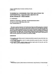
1

Figure 2.1: This gure shows the dierence between the fourth partial sum of (3; 1) P 4 ? 1 biorthogonal wavelets and the weight function in the Haar basis, k=0 4;k (t) ? (t). ?1  (t) See gure(2.1). That is, the dierence between the nth partial sum Pkn=0 n;k and (t) is non-zero on an interval of length 3=2Pn and has largest magnitude equal ?1  (t) converges pointwise to to 2?n+2(59)=2880. We can then conclude that kn=0 n;k

(t) = t ? 1=2, proving our claim. 

2.2.2 Homogenization via Augmentation

We now apply the augmentation procedure of section (2.1.2) to our eective equation. The corresponding homogenized integral equation

Ghx(t) ? = F h has homogenized coecients

!

Gh = 10 01

Zt 0

x(s) ds

!

and F h = 00 M1 ?0 2M2 : 22

This integral equation corresponds to the dierential equations

8 du < dt = (M1 ? 2M2)v : dvdt = 0:

(2.24)

Notice that these are dierent from the homogenized equations for the classical theory (see section 2.3): 8 du < dt = M1 v : dvdt = 0: However, the rst system of dierential equations (2.24) is consistent with the goal of the wavelet-based homogenization. The averages of the solutions to the original equations (the non-constant coecient case) are

Z1 Zt 1 ! hvi = 2 and hui = 1 + 2 0 0 (s) ds dt; note that the initial condition is = ( 1; 2) 2 R2. To compare this with the averages of u and v as determined by Gh and F h, given by 1  hvi = 2 and hui = 1 + 2 2 M1 ? M2 ; notice that

1 M ? M = 1 Z 1 dt ? Z 1 t ? 1=2 dt 2 2 1 2 (t) 0 (t) Z 1 01 ? t = (t) dt; 0

if we now integrate this last integral by parts, we see that it is exactly

2.2.3 Reduction Procedure with Forcing Terms

R 1 R t 0

ds 0 (s)



dt.

Let us now apply the MRA scheme to the general problem given by ! d  du = f (2.25) dx dx where f is no longer taken to be identically equal to zero. Let f be a continuous function on [0; 1]. We now have to include forcing terms p and q in our reduction procedure. With the same notation as in equation (2.2), the equation (2.25) corresponds to the initial choices ! ! 0 0 q(t) = 0 and p(t) = f (t) : 23

The operators G(0n) and F0(n) and their limits G0(1) and F0(1) remain unchanged. Using similar techniques as those above, we calculate the general form of the vectors p(0n) and q0(n) and determine that the limiting behavior of these quantities is ! ! p q ( n ) ( n ) 1 1 and nlim nlim !1 p0 = m1 !1 q0 = m2 where Z1 Zs 1 Z1 1 Zt p1 = (t) sf (s) ds dt + (s ? 1)f (s) (t) dt ds 0 0 0 Z Z Zs Z0 1 t 1 1 q1 = (t ? 1=2) (t) sf (s) ds dt + (1 ? s)f (s) (1=2 ? t) (1t) dt ds

m1 =

Z0 1 0

0

f (t) dt and m2 =

Z1 0

0

0

(t ? 1=2)f (t) dt:

The reduced equations for the averages hui and hvi are hui = 1 + 2( 21 M1 ? M2 ) + ( 21 m1 ? m2)( 21 M1 ? M2 ) + 12 p1 ? q1 (2.26) (2.27) hvi = 2 + 21 m1 ? m2 : If we simplify the expressions (2.26) and (2.27), we have Z 1Z t Z 1Z 1 1 ds dt (1 ? t ) f ( t )(1 ? s ) dt + hui = 1 + 2 0 0 ds (s) !(s) 0 0 Z1 Z Z t 1 + (1 ? t) (1t) sf (s) ds ? (1 ? s)f (s) ds dt 0 0 t Z 1 Z t ds Z 1Z 1 = 1 + 2 dt + (1 ? t)f (t)(1 ? s) 1 ds dt !(s) 0 0 (s) 0 0 Z Z1 Z 1 t + (1 ? t) (1t) (s ? 1)f (s) ds + f (s) ds dt 0 0 0 Z1 Z Z 1 Z t ds 1 t f (s) ds dt (1 ? t ) dt + = 1 + 2 (t) 0 0 0 0 (s) Z 1Z xZ t f (s) Z 1 Z t ds dt + ds dt dx and = 1 + 2 0 0 0 (t) 0 0 (s) Z 1Z t hvi = 2 + f (s) ds dt: 0 0

In other words, the equations (2.26) and (2.27) are indeed the averages of the solutions to equations 2.25) given by Zx Zx u(x) = 1 + v((tt)) dt and v(x) = 2 + f (t) dt: 0 0 24

The corresponding homogenized integral equation

Ghx(t) ? has homogenized coecients Gh and

0 ph = @

1 2

Zt h = F x(s) + ph ds 0 F h as above and the coecient ph 1

p ?q1 M1 ?M2

1 2 1

(2.28) is

+ 31 ( 12 m1 ? m2 )A : m1 ? 2m2

One can verify that the solutions of equation (2.28) given by

Zt

u(t) = 1 + (M1 ? 2M2 ) v(s) + 0 Zt v(t) = 2 + (m1 ? 2m2) ds

1 2 p1 ? q 1 1M ? M 2 2 1

+ 1 ( 1 m1 ? m2 ) ds 3 2

0

have the same averages as the solutions of equation (2.25). We conclude that the homogenized coecients Gh and F h do not depend on the forcing term f , only the homogenized coecient ph depends on our choice of f . Furthermore, the MRA scheme produces a homogenized equation for the general problem (2.25) which preserves the averages of the solution.

2.3 Several approaches in classical homogenization theory: a review In this section we review the classical homogenization theory for one-dimensional elliptic dierential equations. Let  be a periodic function in L1([0; 1]) such that (x)   > 0 for all x 2 [0; 1]. We will associate to  the dierential operator d  d : L = dx dx If we de ne (x) = (x?1 ), then we have an associated family of operators d (x?1 ) d : L = dx dx We also have a family of solutions u in H01([0; 1]) which solve the Dirichlet problems d (x?1 ) du  = f: Lu = dx (2.29) dx 25

A positive constant 0 is the homogenized or eective coecient for this problem if for any f 2 H ?1([0; 1]), the solutions u of the Dirichlet problem (2.29) have the following property: u ! u0 weakly in H01([0; 1]) and du0 weakly in L2 ([0; 1]) as  ! 0;   du !  0 dx dx where u0 is the solution of the Dirichlet problem d  du0  = f for u 2 H 1([0; 1]): 0 0 0 dx dx   The operator dxd 0 dxd is called the homogenized operator and the equation d  du0  = f dx 0 dx is called the homogenized equation. The vector elds p =  dudx ; p0 = 0 dudx are called

ows. Let us derive the value of 0 with two dierent methods: an asymptotic expansion of the solution u in powers of  and a direct examination of the ows p. We want to emphasize that these methods are used for physical problems which have two or more (but nitely many) distinguished scales. We will show that the multiresolution approach can be applied to physical problems with a continuum of scales and as such is more robust. 

2.3.1 Asymptotic Method 



0

In the problem dxd (x?1 ) dudx = f , we have two distinguished scales (the scales of x and x?1 ) so we seek a two-scale asymptotic expansion of the solution u. As a rst approximation, we look for a solution of the form u(x; ) = u0(x) + u1(x; y) where y = x?1 and u1 is periodic with respect to y. Note that dxd = @x@ + 1 @y@ . Then d (y) du  = ?1 ( u +  u ) + ( u +  u ) + ( u ) f = dx 1 1 2 0 3 0 2 1 3 1 dx (2.30) where @ (y) @  1 = @y @y  @ @  + @ (y) @ ; and 2 = @y (y) @x @x @y 2 @ : 3 = (y) @x 2 

26

The rst term in the right-hand-side of equation (2.30) must equal zero, so @ (y) @u1  = ? d du0 : @y @y dy dx This is a periodic boundary value problem in y with the right-hand-side depending on x as a parameter. Let N be the solution of d (y) dN  = ? d : (2.31) dy dy dy Notice that equation (2.31) is equivalent to the problem d (y)(1 + dN ) = 0: (2.32) dy dy Then u1(x; y) = N (y) dudx and u(x) = u0(x) + N (y) dudx . Let us use this fact and the second term in equation (2.30) to determine: 2 d (y)N (y) d2u0 + (y) dN d2 u0 3u0 + 2 u1 = (y) ddxu20 + dy dx2 dy dx2 2  d ((y)N (y)) +  dN : = ddxu20 (y) + dy dy 0

0

Averaging this term with respect to y, we get

d u0 h3u0 + 2 u1i = h(y) + (y) dN dy i dx2 2

2 u0 d = 0 dx2 where 0 = h(y) + (y) dN dy i is our homogenizedR coecient. R From (2.32) we know that N (y) = ?y + M1 0y ds(s) where M1 = 01 ds(s) and so 0 = h(y) ? (y) + M1 )i = M1 = h 11 i ; 1  the harmonic average of . For the justi cation of this method see [15]. 1

1

2.3.2 Flows

In this section we review a dierent approach using the ows p(x) = (x?1 ) dudx . In this one-dimensional caseR these are sucient for us to determine the value of 0. Set B (x) = (1x) and F (x) = 0x f (t) dt. Then the equation can be rewritten as 

du = B (x?1 )F (x) ? c :  p(x) = (x?1 ) du = F ( x ) ? c and   dx dx 27

The constants c, which are indexed by , are determined by our boundary conditions Z1 Z1   0 = du dx = B (x?1 ) F (x) ? c dx: (2.33) 0 dx 0 To nd lim!0 c we must invoke a simple property of periodic functions that is frequently used in homogenization theory. Theorem 2.3.1 Let g : Rn ! C be a periodic function whose period cell is a box B with edges directed along the coordinate axes and edge lengths l1; l2 ; : : : ; ln respectively. We denote the mean value of g by hgi; i.e., Z 1 hgi = jB j B g(x) dx where jB j = l1 l2


ln. The space Lp (B ) is the space of periodic functions with nite norm h jgjpi1=p for p  1. Assume that g 2 Lp (B ); p  1. Then g(x=) ! hgi weakly in Lp ( ) as  ! 0, where is an arbitrary bounded domain in Rn; i.e., g(x=) ! hgi weakly in Lploc (Rn): Proof. We can restrict ourselves to the situation = sB where is a dilation of the basic box B with ratio s  1. Observe that for f 2 Lp(B ) and   1,

Z



jf (x=)jp dx = n

Z



sB 



jf (x)jp dx  n [s?1 ] + 1 nh jf jpi  c0 h jf jpi

for c0 depending on and for bs?1 c the greatest integer not larger than s?1 . Let q be a trigonometric polynomial with the same periodicity as g such that hqi = hgi and h jg ? qjpi  . Then for   1, we also have

Z



jg(x=) ? q(x=)jp dx  c0:

This estimate shows us that it is sucient to prove the result for trigonometric polynomials. However, for trigonometric polynomials this is simply a consequence of the Riemann-Lebesgue lemma.  Now, let us apply the previous result about the mean value to the relation (2.33). In the limit for  ! 0, this gives

hB i

R

Z1 0

F (x) dx ? lim c hB i = 0; !0 

or lim!0 c = 01 F (x) dx. We can now also determine the weak limits in L2 ([0; 1]) of the sequences dudx and p. We have 

Z1

lim p (x) = F (x) ? F (x) dx = p0 (x); !0  0 Z1   du0 du  lim ( x ) = h B i F ( x ) ? F ( x ) dx = dx (x): !0 dx 0 28

These formulas show us that 0 p0(x) = hB1 i du (x) and dp0 (x) = F 0(x) = f (x); dx dx so that u0 is the solution of the Dirichlet problem

! d h?1i?1 du0 = f with u 2 H 1([0; 1]): 0 0 dx dx

Therefore, the homogenized coecient 0 is h?1i?1. We note that the value of 0 for these one-dimensional elliptic equations holds in a much more general context (although we derived the value in the above, more restricted context). In particular, the operators L : H01([0; 1]) ! H0?1([0; 1]) form a sequence of linear operators which are uniformly coercive and uniformly bounded. The sequence of inverses L? 1 : H0?1([0; 1]) ! H01([0; 1]) is bounded uniformly so we may extract a subsequence L? 1 which converges (with respect to the weak topology in the space of operators) to a bounded operator M : H0?1([0; 1]) ! H01([0; 1]). This operator M is coercive and admits an inverse, denoted L0 : H01([0; 1]) ! H0?1([0; 1]). It can be shown that the operator L0 is the homogenized operator with the form dxd 0 dxd with homogenized coecient 0 = h?1i?1. See [15] for a more detailed discussion. We can see from the previous calculations and discussions that we have an explicit value for 0 in one-dimensional elliptic equations. In two or more dimensions it is sometimes possible to determine explicitly the homogenized matrix (see [15] for examples). For cases in which an explicit value cannot be determined, we can apply the Voigt-Reiss Inequality (in [15]). Theorem 2.3.2 If we assume that the initial periodic matrix  is symmetric, then the homogenized matrix 0 satis es the following inequality:

h?1i?1  0  hi: Furthermore, 0 = hi holds only if div  = 0 and h?1 i?1 = 0 holds only if curl ?1 = 0.

2.4 Physical Examples In this section we will present two examples which illustrate the dierences between the classical and the MRA homogenization methods. We will show that the MRA method is more physically robust, meaning with this method we can handle many more physical situations. The physical problem which we will look at is the steady-state heat distribution in a rod of length one. We will assume that the temperature T satis es T (0) = 29

T (1) = . We also assume that the average temperature gradient h dT dx i = R0 1and dT (s) ds = . Our heat equation is then 0 dx ! d  dT = 0 dx dx with the conditions T (0) = 0, T (1) = , and h dT dx i = . Also, the thermal conductivity  is a bounded function, bounded away from zero, and has period one. We will homogenize this problem for several dierent functions . First, we will look at a family of thermal conductivities

n(x) = (2nx): Each function n models a material composed of period cells (of length 2?n) and we want to know the eective thermal conductivity of the material as n ! 1 (or as the length of each period cell shrinks to zero). This is the physical motivation for the classical theory. Theorem 2.4.1 If we use the MRA strategy to homogenize the problem d  dTn  = 0 (2.34) dx n dx for each n and then take the limit as n ! 1 of the homogenized coecients hn, we will replicate the classical homogenization results. Proof. Again, rewriting (2.34) as a system of ODEs gives us dTn = vn and dvn = 0 with T (0) = 0 and v (x) = hv i =  n n n dx n dx M1;n where M1;n =

R1

ds 0 n (s) .

We know from the results of the previous section (2.2) that

  2;n hTni = Tn (0) + vn (0) M21;n ? M2;n = 2 ? M M 1;n

hvni = hvn(0)i = M : 1;n

Here M2;n =

R 1 s?1=2 ds. Furthermore, the homogenized equations are 0 n (s)

Tnh(x) =

Zx

  vnh(s) M1;n ? 2M2;n ds 0 vnh(x) ? M = 0; 1;n 30

or, in dierential form, d (h dTnh ) = 0 with T h(0) = 0 and dTnh (0) =  : n dx n dx dx M1;n The eective coecient is given by hn = M ?1 2M : 1;n 2;n In the limit as n goes to in nity, we have Z 1 ds 1 lim M = lim n!1 1;n n!1 0 (2n s) = h  i and Z1 Z 1 s ? 1=2 1 i (s ? 1=2) ds = 0 ds = h lim M = lim  0 n!1 2;n n!1 0 (2ns) by Theorem (2.3.1). In general, we can conclude that 1 1 h nlim !1 n = nlim !1 M1;n ? 2M2;n = h 1 i ; or that our homogenized coecient is simply the harmonic average of  (the same as the classical theory!).  We will now examine a speci c family of thermal conductivities. Let  1(x) = 2 ? sin(22nx). The moments M1;n and M2;n are Z1 Z1 M1;n =  dx(x) = (2 ? sin(22nx)) dx = 2 0 0 Z1 Z 1 xn? 1=2 n x)) dx = 1 : ( x ? 1 = 2)(2 ? sin(2  2 dx = M2;n =  (x) 22n n

0

n

0

So, hTnhi = 2 (1 ? 212 ) and Tnh(x) = (1 ? 212 )x. Furthermore, our homogenized coecient is hn = M ?1 2M = 2(1 ?1 1 ) : 1;n 2;n 22 The classical theory tells us that our homogenized problem is d ( 1 dT0 ) = d ( 1 dT0 ) = 0 dx M1 dx dx 2 dx with T0 (0) = 0 and T0(1) = . We get T0 (x) = x and hT0i = 2 . Observe that in the limit as n ! 1 the two methods agree; i.e., 1= 1 1 h = lim = lim  n 1 n!1 n!1 2(1 ? 22 ) 2 M1 h(x) = lim (1 ? 1 )x = x: lim T n n!1 n!1 22n n

n

n

n

31

This example prompts a question. Does the MRA strategy provide a higher order correction term in the asymptotic expansion derived in the classical theory? The answer to the question is no, the MRA scheme is not simply a higher order term in the asymptotic expansion of the classical theory. Recall that the classical theory tells us 0 T (x)  T(x) = T0(x) + N (y) dT dx d dN ? n where we take  = 2 and N solves dx ((y)(1 + dy )) = 0 with y = 2nx and R N (0) = N (1) = 0. Here, T0 (x) = x and N (y) = ?y + M1 0y ds(s) . Therefore, 1

T (x)  T2? (x) = T0

(x) + 2?nN (y) dT0

 = x + 2?n ?y +

1 Z y ds  M1 0 (s)

dx Z2x  2 ? sin(2s) ds = 2n M 1 0 n   = x +  cos(22n x) ? 1 n : 2 22 22   So, the correction term is 2 cos(2222 x) ? 212 . The MRA algorithm gives n

n

n

n

n

Tnh(x) = x ? 2x  2n :

It is clear that the MRA scheme does not give us simply a more accurate approximation to the true solution T . The solution Tnh is a linear function which has the same average as the true solution Tn but which tends pointwise to T0 as n goes to in nity. If we graph the dierence of T0 and the two functions T2? and Tnh (see gure2.2), we see that the approximate solution T2? oscillates just below the line T0 (x) = x and as n tends to in nity these oscillations increase in frequency and decrease in amplitude. The function Tnh is a straight line from the origin to the point (1; (1 ? 1 h 22 )) with its average value exactly equal to the average of Tn . Also, in the limit Tn is the line x. As we discussed previously, the MRA scheme is more physically robust than the classical theory. The next example will illustrate a situation that falls outside of the reach of classical theory and yet, physically, this is an important case we would like to homogenize. This example is a problem with a continuum of scales. Let 1 = 2 ? sin(2 tan(  x)) (x) 2 n

n

n

(see gure 2.3). This conductivity corresponds to a material composed of period cells but which has been stressed or distorted at one end. We emphasize that there is no 32

0 MRA homogenized solution asymptotic solution -0.002 -0.004 -0.006 -0.008 -0.01 -0.012 -0.014 -0.016 -0.018 -0.02 0

0.1

0.2

0.3

0.4

0.5

0.6

0.7

0.8

0.9

1

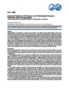
Figure 2.2: This gure shows a comparison of the dierence between the MRA homogenized solution and the true solution Tnh(x) ? x (in the dotted line
) on one hand, and of the dierence between the asymptotic solution and the true solution T2? (x) ? x (in the dashed line -). Here n = 3 and  = 1. Both of the functions Tnh and T2? correspond to the temperature in a rod with period cells of length 2?n. n

n

small parameter  (or family of thermal conductivities n(x) = (2nx)) unlike the previous examples. We can calculate Z1 M1 = 2 ? sin(2 tan( 2 x)) dx  1:89173 and Z0 1 M2 = (x ? 1=2)(2 ? sin(2 tan( 2 x)) dx  0:05225: 0

These quantities allow us to determine the average temperature distribution hT i and to write an homogenized equation for this example even though there is no small parameter in which we could do an asymptotic expansion as in the classical theory.

33

1 0.8 0.6 0.4 0.2 0 −0.2 −0.4 −0.6 −0.8 −1 0

0.1

0.2

0.3

0.4

0.5

0.6

0.7

0.8

0.9

Figure 2.3: This is a plot of the thermal conductivity (1x) = 2 ? sin(2 tan( 2 x)). This function \contains" a continuum of scales.

2.5 Conclusions The MRA strategy for numerical homogenization consists of two algorithms; a procedure for extracting the eective equation for the average or for the coarse-scale behavior of the solution (the reduction process) and a method for augmenting this effective equation (the augmentation process). In other words, once one has determined what the average behavior of the solution is, one can construct a simpler equation whose solution has the same average behavior. For physical problems in which one wants to determine only the average behavior of the solution, the reduction process is very useful and is not part of the classical theory of homogenization. In some applications, this step suces. On the other hand, the augmentation procedure yields eective material parameters (or homogenized coecients) just as the classical theory does; however, the MRA procedure produces a homogenized equation which preserves important physical characteristics of the original solution, such as its average value. The MRA method is more physically robust in that it can be applied to many more situations than the classical theory can. For example, the MRA strategy can be applied to problems which have a continuum of scales while the classical theory may be applied to problems with only a nite number of distinguished scales. Moreover, for those two-scale problems for which the classical theory was developed the MRA results agree with the results of classical homogenization in one dimension. 34

Chapter 3 MRA Reduction Methods for Nonlinear ODEs Let us begin by highlighting the diculty in the reduction procedure for nonlinear equations. The reduction procedure begins with a discretization of the nonlinear equation. Just as the initial discretization of a linear ODE is a linear algebraic system, the initial discretization of a nonlinear ODE is a nonlinear system F (x) = 0: (3.1) The nonlinear function F maps RN to RN (for N = 2n) and we denote the kth coordinate of F (x) by F (x)(k). Similarly, we denote the kth coordinate of x by x(k). We change basis by writing     s(k) = p1 x(2k + 1) + x(2k) and d(k) = p1 x(2k + 1) ? x(2k) ; 2 2 the averages and dierences of neighboring entries in x. We split our equation into two equations in the two unknowns s and d by applying Ln and Hn to equation (3.1). The 2n?1  2n matrix Ln is the top half of the matrix Mn and 2n?1  2n matrix Hn is the bottom half of 0 1 1 1 0 0 : : : BB 0 0 1 1 0 0 : : :CC BB CC ... B CC 1 Mn = p B B CC : ? 1 1 0 0 : : : 2B BB 0 0 ?1 1 0 0 : : :CC @ A ... Our two equations are   Ln F (s; d) = 0 (3.2)   Hn F (s; d) = 0: (3.3) 35

Notice that the function LnF maps RN=2  RN=2 to RN=2 and similarly for HnF but that we cannot split these functions into their actions on Lnx = s and Hnx = d (as we did in the linear case). Instead, we can give the coordinate values for Ln F and Hn F :     LnF (s; d) (k) = p1 F (s; d)(2k + 1) + F (s; d)(2k) 2     1 HnF (s; d) (k) = p F (s; d)(2k + 1) ? F (s; d)(2k) 2 for k = 0; : : : ; 2n?1 ? 1. As with the linear algebraic system, we must eliminate the dierences d from the nonlinear system (3.2-3.3). In other words, we must solve equation (3.3) for d as a function of s. This equation, however, is a nonlinear equation and may not be easily solved (if at all). Let us assume that we can solve equation (3.3) for d as a function of s and let d~(s) denote the solution. We then plug d~(s) into equation (3.2) to get LnF (s; d~(s)) = 0 which is the reduced equation for the coarse behavior of x. The form of the original system is preserved under this procedure and we may write the recurrence relation for F as follows: Fj?1(s) = Lj Fj (s; d~(s)) where d~(s) satis es Hj Fj (s; d~(s)) = 0. In the following two sections we will  give the precise form of the nonlinear system (3.3){(3.2) in d and s,  state conditions for (3.3){(3.2) under which we can solve for d as a function of s,  develop two approaches for solving (3.3){(3.2) for d (a numerical and an analytic approach), and  derive formal recurrence relations for the nonlinear function Fj .

3.1 Nonlinear Reduction Method We now extend the MRA reduction method to nonlinear ODEs of the form

x0 (t) = F (t; x(t)); t 2 [0; 1]:

(3.4)

We will address the diculties raised in the previous section with two approaches, a formal method to be implemented numerically and an asymptotic method. We 36

will assume that F is dierentiable as a function of x and as a function of t. The assumption that F is Lipschitz as a function of x guarantees the existence of uniqueness of the solution x(t). For the reduction procedure F must be Lipschitz in t and dierentiable in x. We will rewrite this dierential equation as an integral equation in a slightly unusual form:

G(t; x(t)) ? G(0; x(0)) =

Zt 0

F (s; x(s)) ds;

(3.5)

where @g=@x 6= 0. The more usual dierential equation (3.4) is obtained by setting G(t; x(t)) = x(t) and by dierentiating. We choose this integral formulation because we can maintain this form under the reduction procedure. In our derivations we nd it helpful to use an operator notation in addition to the coordinate notation so we write equation (3.5) in an operator form,



G(x) = K F(x) where



(3.6)

Zt

K(y)(t) = 0 y(s) ds; G(y)(t) = G(t; y(t)); and F(y)(t) = F (t; y(t)): We will use the MRA of L2 ([0; 1]) associated with the Haar basis to begin our discretization. We discretize equation (3.6) in t by applying the projection operator Pn to equation (3.6) and seeking a solution xn 2 Vn to the equation

Gn(xn) = KnFn (xn)

(3.7)

where

Gn(xn) = PnG(xn); Kn = PnKPn; and Fn(xn ) = PnF(xn): Because we are using the Haar basis, xn is a piecewise constant function with step width n = 2?n. The functions Gn(xn) and Fn(xn ) are also piecewise constant functions. Note that Gn, Fn, and Kn map Vn to Vn, although Gn and Fn are nonlinear functions. Let xn(k) denote the value of the function xn on the interval kn < t < (k +1)n, for k = 0; : : : ; 2n ? 1. Let gn(xn )(k) and fn(xn)(k) denote the values of the functions Gn(xn) and Fn (xn) on the same interval. That is,

Z (k+1)   1 gn(xn)(k) =  g(s; xn(k)) ds = PnG(xn) (t) n k where kn < t < (k + 1)n, and similarly for fn(x)(k). We can say that gn(xn)(k) is the average value of the function G(t;
) over the time interval (kn; (k + 1)n) and evaluated at xn (k). Notice that gn(xn)(k) is shorthand for gn(xn (k))(k). n

n

37

As in [9] we use the integration operator Kn de ned by

01 BB 2 BB1.. Kn = n B @.

0 ... ...




01C

... ... 1


1

... C CC : 0C A

(3.8)

1 2

With this notation, the coordinate form of equation (3.7) is

gn(xn )(k) = n

kX ?1 k0=0

fn(xn )(k0) + 2n fn(xn)(k):

(3.9)

This equation gives the precise form of the nonlinear system F (x) = 0 discussed in the previous section. We are now ready to begin the reduction procedure. We rst split the equation (3.7) into two equations, one with values in Vn?1 and the other with values in Wn?1, by applying the projection operators Pn?1 and Qn?1. We now have the two equations

  Pn?1Gn(xn) = Pn?1Kn Fn(xn)   Qn?1Gn(xn) = Qn?1 Kn Fn(xn ) :

(3.10) (3.11)

At this point let us work with two consecutive levels and drop the index n indicating the multiresolution level (assume that  = n). We recall that for the Haar basis the action of the operators Pn?1 and Qn?1 amounts to forming averages and dierences of the odd and even elements of a vector (renormalized by a factor of p 2). We will modify the Haar basis slightly and normalize the dierences by 1=. The averages will not be adjusted by any factor. By forming successive averages of equation (3.9), we can rewrite equation (3.10) in coordinate form as 2k 1 g(x)(2k + 1) + g(x)(2k) =  X 0 ) +  f (x)(2k + 1) f ( x )( k 2 2 k0=0 4 2X k?1 f(x)(k0 ) + 4 f(x)(2k): + 2 k0 =0

(3.12)

In the same manner we rewrite equation (3.11) by taking successive dierences normalized by the step size : 1 g(x)(2k + 1) ? g(x)(2k) = 1 f(x)(2k + 1) + f(x)(2k): (3.13)  2

38

Let us rearrange the right hand side of equation (3.12) as follows: 2k 2X k?1 X   0 0 ) +  f (x)(2k) f ( x )(2 k + 1) + f ( x )( k ) + f ( x )( k 2 k0=0 4 2 k0=0 4 2X k?1 =  f(x)(k0 ) + 4 f(x)(2k + 1) + 34 f(x)(2k) k0 =0 kX ?1     f(x)(2k0 + 1) + f(x)(2k0) + 2 f(x)(2k + 1) + f(x)(2k) = k0 =0   ? 4 f(x)(2k + 1) ? f(x)(2k) : To simplify our notation, let us de ne S and D as \average" and \dierence" operators which act on g(x) and f (x) by taking successive averages and dierences of elements g(x)(k) and f (x)(k). We de ne S and D as follows:   Sg(x)(k) = 21 g(x)(2k + 1) + g(x)(2k)   Dg(x)(k) = 1 g(x)(2k + 1) ? g(x)(2k) : Then we may write the coordinate form of equations (3.10-3.11) in a compact form kX ?1 2 Sg(x)(k) + 4 Df (x)(k) = 2 Sf (x)(k0 ) + Sf (x)(k) (3.14) k0=0 Dg(x)(k) = Sf (x)(k) (3.15) We have split the equation (3.9) into two sets and now we split the variables accordingly. We de ne the averages sn?1 and the scaled dierences dn?1 as     sn?1(k) = 21 xn (2k + 1) + xn (2k) and dn?1(k) = 1 xn(2k + 1) ? xn(2k) : Notice that since xn is a piecewise constant function with step width n, then sn?1 and dn?1 are piecewise constant function with step width 2n = n?1 . We will now change variables in equations (3.14) and (3.15) and replace x with x(2k + 1) = s(k) + 2 d(k) and x(2k) = s(k) ? 2 d(k): We will abuse our own notation slightly for clarity and denote the change of variables by   Sg(s; d)(k) = 21 g(s + 2 d)(2k + 1) + g(s ? 2 d)(2k)   Dg(s; d)(k) = 1 g(s + 2 d)(2k + 1) ? g(s ? 2 d)(2k) :

39

Note that when we write g(x)(k), this is shorthand for g(x(k))(k); so g(x)(2k + 1) stands for g(x(2k + 1))(2k + 1). When we replace x(2k + 1) with s(k) + 2 d(k) and write g(x)(2k + 1) = g(s + 2 d)(2k + 1), this is shorthand for the expression g(x(2k + 1))(2k + 1) = g(s(k) + 2 d(k))(2k + 1): The shorthand notation g(s ? 2 d)(2k) is similar. Then our system of two equations in the two variables s and d is given by kX ?1 2 Sg(s; d)(k) + 4 Df (s; d)(k) = 2 Sf (s; d)(k0 ) + Sf (s; d)(k) k0=0 (3.16) Dg(s; d)(k) = Sf (s; d)(k) (3.17) Our goal, as in the linear case, is to eliminate the variables d from equations (3.16-3.17) to obtain a single equation for s. We consider (3.17) as an equation for d which we have to solve in order to nd d in terms of s. Let us assume that we can solve (3.17) for d and let d~ represent this solution. Notice that equation (3.17) is a nonlinear equation for d so that d~ is a nonlinear function of s. We will discuss how this is implemented numerically in the section 3.4 and how this is implemented analytically in section 3.2. In the linear case, d~ is a linear function of s and it can be easily computed explicitly. Provided that we have d~, we substitute this into equation (3.16) and obtain kX ?1 2 Sg(s; d~)(k) + 4 Df (s; d~)(k) = 2 Sf (s; d~)(k0 ) + Sf (s; d~)(k) k0=0 (3.18) Observe that we may arrange equation (3.18) as follows kX ?1 gn?1(k)(sn?1) = n?1 fn?1 (k0)(sn?1) + n2?1 fn?1(k)(sn?1) (3.19) 0 k =0 where 2 gn?1(k)(sn?1) = Sgn(k)(sn?1; d~n?1) + 4n Dfn(k)(sn?1; d~n?1) and (3.20) fn?1 (k)(sn?1) = Sfn(k)(sn?1; d~n?1) (3.21) In other words, the reduced equation (3.19) is the eective equation for the averages sn?1 of xn. It is important to note that this equation has the same form as the original discretization. Let us switch now to operator notation to present the recurrence relations for the reduction procedure. We use the solution d~ of equation (3.17) to write equation (3.19) in operator form as G(nn?)1(sn?1) = Kn?1 Fn(n?)1(sn?1) 40

where sn?1 = Pn?1x and the nonlinear operators G(nn?)1 and Fn(n?)1 map Vn?1 to Vn?1. The superscript (n) on the operators denotes the level at which we start the reduction procedure and the subscript n ? 1 denotes the current level of resolution. The operators Gn(n?)1 and Fn(n?)1 are de ned as the operators which act elementwise according to equations (3.20) and (3.21), respectively. Notice that they have the same form as the operators G(nn) and Fn(n) ; both functions G(nn?)1(sn?1) and Fn(n?)1(sn?1) are piecewise constant functions with step width n?1. In particular, the k-th element of G(nn?)1(sn?1) depends only on the arguments through the k-th element of sn?1(k). Because the form of the discretization is preserved under reduction, we can consider the equations (3.21) and (3.20) as recurrence relations for the operators G(nn?)1 and Fn(n?)1 and, as such, may be applied recursively to obtain a sequence of operators G(jn) and Fj(n), j  n. The recurrence relations for G(jn) and Fj(n) (for j  n) in operator form are given by j2+1 (n) ( n ) ( n ) Gj = Pj Gj+1 + 4 Qj Fj+1 (3.22) n) ; Fj(n) = Pj Fj(+1 (3.23) n) exists. Observe that the provided the solution d~j of the equation Qj G(jn+1) = Pj Fj(+1 operator forms of the \average" and \dierence" operators S and D, which we introduced in working with the coordinate forms of our expressions, are the projections Pj and Qj . We emphasize that this is a formal derivation of the recurrence relations. We show in section 3.4 how to implement numerically this formal procedure. In section 3.2 we derive analytic expressions for these recurrence relations. Let us now address the existence of the solution d~j to the equation Qj G(jn+1) = n) . We will write this equation in coordinate form as follows (dropping subPj Fj(+1 scripts): F (s; d)(k) = Dg(s; d)(k) ? Sf (s; d)(k) = 0 2 where F : E ! R , (s; d) 2 E an open set in R2  R2 , and k = 0; : : : ; 2j ? 1. Assume that g and f are both dierentiable functions so that F 2 C 1 (E ). Suppose that there is a pair (s0; d0) 2 E such that F (s0; d0)(k) = Dg(s0; d0)(k) ? Sf (s0 ; d0)(k) = 0 and that the Jacobian of F with respect to d at (s0; d0) does not vanish. (We know that such a pair (s0; d0) 2 E must exist since a unique solution to our ODE exists.) The Implicit Function Theorem tells us that there is a neighborhood S of s0 in R2 and a unique function d~: S ! R2 (d~ 2 C 1 (S )) such that d~(s0 ) = d0 and F (s; d~(s)) = 0 for s 2 S . Let us investigate what it means for the Jacobian of F with respect to d at (s0; d0) to be nonzero. Notice that the k-th coordinate of F , F (s; d)(k), depends only on the k-th coordinates of s and d F (s; d)(k) = Dg(s; d)(k) ? Sf (s; d)(k): j

j

j

j

j

41

In turn, s(k) and d(k) depend on x(2k + 1) and x(2k) and we may write F (s; d)(k) in terms of x(2k + 1) and x(2k). In particular, we can write   Dg(s; d)(k) = 1 g(x)(2k + 1) ? g(x)(2k)   Sf (s; d)(k) = 21 f (x)(2k + 1) + f (x)(2k) where x(2k + 1) = s(k) + 2 d(k) and x(2k) = s(k) ? 2 d(k): When we dierentiate F (s; d)(k) with respect to d(k), we can apply the chain rule and dierentiate with respect to x(2k + 1) and x(2k) instead. Therefore, the derivative of the term Dg(s; d)(k) with respect to d(k) is @ Dg(s; d)(k) = 1 dg(x)(2k + 1) + 1 dg(x)(2k) = Sg0(s; d)(k): @d(k) 2 dx(2k + 1) 2 dx(2k) We calculate a similar expression for the derivative of Sf (s; d)(k). Hence, the Jacobian of F with respect to d is given by the matrix JF with entries (k; l):

F (k) = @ Dg(s; d)(k) ? Sf (s; d)(k) JF (s; d)(k; l) = @@d 8 (l0 ) d(l)  0 Rd, the series is divergent. To have a convergent series C must satisfy (1 + C ) < 22(j+1) , which C does indeed satisfy. Using this estimate, we examine the series for gj(n) and fj(n) . Let us assume that kPj i;j(n)+1k and kQj (i(?n)(l+1);j+1 )0k are uniformly bounded by C 0. Then we can bound

61

i;j(n) by

ki;j?1

k  C0

! i?1 X C (1 + C 0 =4)(1 + C )l?1 ? i ? ( i +1)+ l 4 + 4 l=0

i?1 X

 C 0 4?i + 4?i (1 + C )l?1 l=0

!

4l

00  C4i (1 + C )i: We calculate the radius of convergence of fj(n) and nd that C must satisfy the same condition (1 + C )  22(j+1) for fj(n) to converge. A similar calculation holds for gj(n) with the same result. 

62

3.4 Implementation and Examples In this section we present the numerical implementation of our formal reduction procedure, which we derived in section (3.1), and three examples to evaluate the accuracy of our reduction methods and to explore \patching" together the series expansion of the recursion relations and the numerical reduction procedure. We also determine numerically the long-term eect of a small perturbation in a nonlinear forced equation.

3.4.1 Implementation of the Reduction Procedure

We initialize our numerical reduction procedure with two tables of values, one table for each of the discretizations of the functions F and G at the starting resolution level n. The rst coordinate k in our table enumerates the averages in time of the functions F and G, the functions gn(sn)(k) and fn(sn)(k), for k = 0; : : : ; 2?n ? 1. Notice that these are still functions of sn which is unknown, so we also discretize in sn. In other words, from the start, we look at a range of possible values sn(k; i) (i = 0; : : : ; N ? 1) for each k, and work with all of them together. This discretization gives us the second coordinate i for our tables. We then have the values gn(sn(k; i))(k) and fn(sn(k; i))(k) for k = 0; : : : ; 2n ? 1 and i = 0; : : : ; N ? 1. To look at a range of possible values in sn(k), we must have some a priori knowledge of the bounds on the solution of the dierential equation. Next we form the equation (dropping the subscript n) which determines d~ on the interval kn?1 < t < (k + 1)n?1 (see equation (3.17)): Dg(s(k; i); d(k; i))(k) = Sf (s(k; i); d(k; i))(k): (3.42) Notice that this is a sampled version of equation (3.17) and for each sample value s(k; i) and for each k = 0; : : : ; 2n?1 ? 1 we must solve (3.42) for d~(k; i). That is, our unknowns d~(k; i) form a two-dimensional array. To solve for each d~(k; i) we must interpolate among the known values g(s(k; i))(k) since we need to know the value g(s(k; i) + 2 d~(k; i))(2k + 1) (and similarly for g(s(k; i) ? 2 d~(k; i))(2k)) and we only have the values at the sample points s(k; i) for i = 0; : : : ; N ? 1. For higher order interpolation schemes, we need fewer grid points in s to achieve a desired accuracy which reduces the size of the system with which we have to work. Once we have computed the values d~(k; i), we calculate the reduced tables of values gn?1(s(k; i))(k) and fn?1(s(k; i))(k), where k = 0; : : : ; 2n?1 ? 1 and i = 0; : : : ; N ? 1, according to the sampled versions of the recurrence relations (3.20{ 3.21): 2 gn?1(s(k; i))(k) = Sgn(k)(s(k; i); d~(k; i)) + 4n Dfn(k)(s(k; i); d~(k; i)) fn?1(s(k; i))(k) = Sfn (k)(s(k; i); d~(k; i)): Notice that the tables are reduced in width in k by a factor of two and that this procedure can be applied repeatedly. 63

Remark Observe that when i = 0 (respectively, i = N ? 1), we cannot interpolate to calculate the values g(s(k; i) ? 2 d~(k; i)) (respectively, g(s(k; i) + 2 d~(k; i))). We must

either extrapolate (and then ignore the resulting \boundary eects" which propagate through the reduction procedure) or adjust the grid in the s variable at each resolution level. An alternate approach could be to use asymptotic formulas valid for large s. We implemented this algorithm in Matlab as a prototype to test the following examples.

3.4.2 Examples

With the rst example we verify our numerical reduction procedure and determine how the accuracy of the method depends on the step-size n = 2?n of the initial discretization. We also evaluate the accuracy of the linear versus cubic interpolation in the context of our approach. We use a simple separable equation

x0 (t) = (1=) x2(t) cos(t=) and x(0) = x0

(3.43)

with the solution available analytically. We observe that the solution x(t) to equation (3.43) exhibits behavior at two scales. We choose  = 1=(4) and the initial value x0 = 1=2. The exact solution is given by 0 x(t) = 1 ? x xsin( t=) : 0 which we use to verify our reduction procedure. In particular we check if the averages of x(t) satisfy the dierence equation derived via reduction. Let us assume that we reduce to resolution level j = 2?j so that we have two tables of values for fj (s(k; i))(k) and gj (s(k; i))(k). If xj (k) is the average of x over the interval k2j < t < (k + 1)2j , then the following equation should hold

gj (xj )(k) = j

kX ?1 k0 =0

fj (xj )(k0) + 2j fj (xj )(k):

We denote by ej (k) the error over each interval kj < t < (k + 1)j and de ne ej (k) by kX ?1  j 0 ej (k) = gj (xj )(k) ? j fj (xj )(k ) ? 2 fj (xj )(k) : k0 =0

Note that we have only sampled values for gj (s(k; i))(k) and fj (s(k; i))(k) and so we must interpolate among these values to calculate gj (xj )(k) for a speci c value xj (k). We want to know how the errors ej (k) depend on the level of resolution at which we begin the reduction procedure. We reduce to resolution level with j = 2?1 and calculate the errors ej (0) and ej (1) using the averages xj (0) = xj (1) = 0:5774. We x the number of sample points in s to be 50 and use linear interpolation. Table (3.1) lists 64

initial resolution = n average error 2?2 0:0774 ? 3 2 0:0290 2?4 0:0069 ? 5 2 0:0019 Table 3.1: Errors as a function of the initial resolution the errors as a function of the initial resolution. If we exclude the errors associated with the initial resolution n = 2?2 and plot the logarithm of the remaining errors as a function of log(n), the slope of the tted line is 1:9660. We can conclude that the accuracy of our numerical reduction scheme increases with the square of the initial resolution. As we described above, we must interpolate between known function values in the tables. We can use the built-in Matlab linear or cubic interpolation routines. We would like to know how the interpolation aects the error of the method and the minimum number of sample points in s we need for both interpolation methods. We use equation (3.43) again with the same values for x0 and . We x the initial resolution at n = 2?5. For technical reasons, with cubic interpolation we can reduce only to resolution level j = 2?2. Table (3.2) list the errors as a function of the number of sample points in s for both linear and cubic interpolation. In Figure (3.2) No. of sample points in s 6 10 15 25 30 50

average error linear cubic 0.0238 0.0045 0.0098 0.0020 0.0052 0.0020 0.0029 0.0020 0.0024 || 0.0019 ||

Table 3.2: Error as a function of the number of sample points in s, with linear interpolation and with cubic interpolation we have plotted the average error as a function of the number of sample points in s for the two methods of interpolation. We can see that with cubic interpolation the minimum number of grid points in s is 15 and that with linear interpolation we can achieve the same accuracy with 50 grid points. We can also see from the graph that increasing the number of grid points (past 15) will yield no gain in the accuracy of the cubic interpolation method. 65

0.025 linear interpolation cubic interpolation

0.02

error

0.015

0.01

0.005

0 5

10

15

20

25 30 grid points in x

35

40

45

50

Figure 3.2: The error as a function of the number of sample points in s for linear and cubic interpolation methods In the second example we will combine the analytic reduction procedure with the numerical procedure. We begin at a very ne resolution n = 2n and reduce analytically to a coarser resolution level n = 2n . From this level we reduce numerically to the nal coarse level j . The analytic reduction procedure is computationally inexpensive compared to the numerical procedure and we want to take advantage of this eciency as much as possible. However, we must balance computational expense with accuracy. With this example we will determine the resolution level n at which this balance is achieved. Again we use a separable equation given by x0 (t) = x2 (t) cos(t=); x0 = 0:1;  = 41 : (3.44) The solution to equation (3.44) is 0 x(t) = 1 ? x xsin( t=) : 0 We begin with analytic reduction at resolution n = 2?10 . We choose the nal resolution level to be j = 2?2 and we let n1 , the resolution as which we switch to the 0

1

0

1

1

0

66

numerical procedure, range from 2 to 5. Table (3.3) lists the errors as a function of n1 . Note that we have used cubic interpolation and ten grid points in x. Figure (3.3) is intermediate resolution = n1 average error 2?2 0:00106 2?3 0:00093 ? 4 2 0:00092 ? 5 2 0:00092 Table 3.3: Errors as a function of the intermediate resolution

0.00106

"errors"

0.00104

0.00102

0.001

0.00098

0.00096

0.00094

0.00092 0

0.05

0.1 0.15 intermediate resolution

0.2

0.25

Figure 3.3: The error as a function of the intermediate resolution level at which we switch from the analytic reduction method to the numerical reduction method. a graph of the average error as a function of the intermediate resolution. We can see from this graph that the biggest gain in accuracy occurs at the intermediate resolution n = 2?3. In other words, at the ner intermediate levels (n1 = 4; 5) we get a small gain in accuracy compared to the computational expense of the additional resolution 1

67

levels in the numerical reduction. To balance accuracy with computational time for this particular example, we should reduce analytically to resolution n = 2?3 and then switch to the numerical reduction to reach the nal level j = 2?2 . The analytic procedure allows us to reduce our problem with very little computational expense (compared to the numerical procedure) and then for the additional accuracy needed we can use only one relatively more expensive numerical reduction step. The third example we will consider is the equation   x0(t) = 1 ? x2 (t) x(t) + A sin(t=); x(0) = x0 ; (3.45) where  is a small parameter associated to the scale of the oscillation in the forcing term. If the amplitude A = 0, then the solution x(t) has one unstable equilibrium point at x0 = 0 and two stable equilibria at x0 = ?1; 1 (see Figure (3.4)). 1

1.5

1

x(t)

0.5

0

−0.5

−1

−1.5 0

0.5

1

1.5

2

2.5 t = time

3

3.5

4

4.5

5

Figure 3.4: The ows for equation (3.45) with zero forcing. A small perturbation in the forcing term will aect large changes in the asymptotic behavior as t tends to in nity. Therefore, the behavior of the solution on a ne scale will aect the large scale behavior. In particular, if the amplitude A is nonzero but small, then the solution x(t) has three periodic orbits. Two of the periodic orbits are stable while one is unstable (see Figure (3.5)). As we increase the amplitude A, there is a pitchfork bifurcation { the three periodic orbits merge into one stable periodic 68

orbit (see Figure (3.6)). We would like to know if we can determine numerically the initial values of these periodic orbits from the reduction procedure and if those periodic solutions are stable or unstable. We will compare these results derived from 1.5

1

0.5

0

−0.5

−1

−1.5 0

0.5

1

1.5

2

2.5

3

3.5

4

4.5

5

Figure 3.5: The ows for equation (3.45) with small but nonzero forcing. Notice that there are three periodic orbits, two stable and one unstable. the reduction procedure with those from the asymptotic expansion of x for initial values near x0 = 0 and for small . Let us begin with the asymptotic expansion of x for small values of . Assume we have an expansion of the form

x(t; )  0 + x1 (t;  ) + 2 x2(t;  ) + : : :

(3.46)

where the fast time scale  is given by  = t=. If we substitute the expansion (3.46) into the equation (3.45), we have the equation @x1 +  @x1 + @x2  = A sin  + x + O(2): 1 @ @t @ Equating terms of order one in , we have @x@ = A sin  , which has the solution x1 (t;  ) = ?A cos  + !(t). The function ! is determined by a secularity condition which we impose on the terms of order . Equating the terms of order  gives us the 1

69

3 2.5 2 1.5 1 0.5 0 −0.5 −1 −1.5 −2 0

0.1

0.2

0.3

0.4

0.5

0.6

0.7

0.8

0.9

1

Figure 3.6: The ows for equation (3.45) with large amplitude A. Notice that there is only one (stable) periodic orbit in this diagram as the system has undergone a pitchfork bifurcation. equation

@x2 = ?A cos  + !(t) ? !0(t): @ The non-oscillatory term ! ? !0 in the above equation is \secular" because if it were non-zero, we would have a linear term in  which is incompatible with the assumed form of the expansion (3.46). Therefore, we set this term equal to zero, ! ? !0 = 0, and determine that !(t) = C1 et. So we have obtained an asymptotic expansion for x   (3.47) x( ; )  0 +  ?A cos  + C1 et : Note that this asymptotic expansion is valid only for t  j log j. We can, however, determine the behavior of x for large time by examining the direction of the growth in x since the direction signi es which stable periodic orbit (1 or ?1) captures the solution. Observe that the sign of the coecient C1 depends on the initial value x0 . In particular, if x0 > ?A then C1 > 0 and if x0 < ?A then C1 < 0. In other words, if  is suciently small, there is a separation point x0 , de ned as the largest value such that if x0 < x0 , then x(t) < 0 as t tends to in nity. According to the asymptotic 70

expansion (3.47), the separation point x0 as  goes to zero is given by

x0  ?A: This is an approximation of the initial value of the unstable periodic solution. Let us derive another approximation for the separation point by linearizing the equation (3.45) about x0 = 0. The linearized dierential equation is the equation

x0 (t) = x(t) + A sin(t=); x(0) = x0; which has the solution x(t) given by

x(t) = et

R



x0 +

Zt 0

 A e?s sin(s=) ds :

The sign of the factor x0 + 0t Ae?s sin(s=) ds as t tends to in nity determines the direction of growth in x(t). In other words, the separation point x0 is the value for which the following is true

Zt  lim x + A e?s sin(s=) ds = 0: t!1 0 0

If we evaluate the integral in the above expression, we determine that x0 satis es

   + A e?t sin(t=) ? A e?t cos(t=) ? 1 = 0: lim x 0 t!1 1 + 2 1 + 2 2

Thus the separation point is given by x0 = 1?+A2 for  suciently small. We have derived two approximations for the initial value near x0 = 0 of the unstable periodic orbit . We will compare these two approximations with the values we determine numerically from the reduction procedure. We now turn to the numerical reduction procedure. Assume that we can reduce the problem to a resolution level j = 2?j where it no longer depends on time (i.e., the problem is now autonomous). This means that the tables gj (s(k; i))(k) and fj (s(k; i))(k) depend only on i and not on k. Let xj (k) denote the average of the solution x over the interval kj < t < (k + 1)j . Observe that for equation (3.45) the functions G and F are given by

  G(t; x(t)) = x(t) ? x0 and F (t; x(t)) = 1 ? x2 (t) x(t) + A sin(t=)

so that the initial value x0 is simply a parameter in the numerical reduction scheme and we may take G(t; x(t)) = x(t). 71

If the solution x(t) is periodic and if j is an integer multiple of that period, the averages xj (k) will be all equal to the value xe (call that the average); that is, xj (1) = xj (2) =


= xe. Therefore the value of gj (
)(k) at each average xj (k) is the same: gj (xj )(1) = gj (xj )(2) =


= gj (xe): Since this holds for all k, we will drop the parameter. We will also drop the subscript j for clarity. If we take the expressions for g evaluated at two successive averages x(l) and x(l + 1) and subtract them, we nd that f (xe) must satisfy

!  0 = g(xe) ? g(xe) = g(x(l + 1)) ? g(x(l)) = 2 f (x(l + 1)) + f (x(l)) = f (xe): This gives us a criterion for nding the average value xe. We know that the average value of the periodic solution x is a zero of f . Finally, the separation point x0 is the initial value such that g(xe) ? x0 = 0. To determine if the separation point x0 is stable or unstable, we will perturb it by a small value . Set the new initial value x0 equal to x0 + . Let (
xe)l denote the deviation from the average value xe in the average of x over the interval lj < t < (l + 1)j . Then, the discretization scheme relates the dierence between (
xe )l and (
xe)l+1: !  g(xe + (
xe)l+1) ? g(xe + (
xe)l ) = 2 f (xe + (
xe)l+1 ) + f (xe + (
xe)l ) :

If we linearize the above equation, the following holds:     g0(xe) (
xe)l+1 ? (
xe )l = 2 f 0(xe) (
xe)l+1 + (
xe)l ; or equivalently, we may use the ratio (
xe)l+1 = g0(xe) + 2 f 0(xe ) : (
xe)l g0(xe) ? 2 f 0(xe)

to test the stability of the separation point x0 . Table (3.4) below lists several values for , the amplitude A, and the corresponding average values xe for the periodic orbits, separation points, and ratios. The separation point which has a corresponding ratio greater than one is the unstable periodic orbit with initial value x0. We reduce to a level where the problem is autonomous and use cubic interpolation. We compare the calculated separation points with those determined by the two analytic methods. The rst number in the errors column is the error in the asymptotic method and the second number is the error in the linear method. Notice that for the values A = 40 and  = 1=(8) we have only one stable periodic solution. In other words, the two stable periodic orbits have merged with the 72

unstable one to create one stable periodic solution. Clearly, this merging of solutions shows that the ne scale behavior of the solution has a large eect on the coarse scale (or long time) behavior. Furthermore, we have detected numerically this large eect. Note that we had to resort to a dierent asymptotic expansion from the one used previously to determine the separation point for A = 40 and  = 1=8.



A

1 16

1

1 16 1 16

10 20

1 8

1

1 8

40

xe 4:0  10?7 1:0006 ?1:0006 4:0  10?6 0:9746 ?0:9746 4:0  10?6 0:8927 ?0:8927 3:0  10?6 0:9991 ?0:9991 ?1:4  10?5

sep. pts ?0:0199 0:9807 ?1:0204 ?0:1989 0:7759 ?1:1732 ?0:3978 0:4951 ?1:2901 ?0:0397 0:9595 1:0387 ?1:5891

ratios x0 (asymp.) x0 (lin.) 1:1354 0:7796 ?1:989  10?2 ? 161 0:7796 1:1276 0:7868 ?0:1989 ? 1610 0:7868 1:1056 0:8185 ?0:3978 ? 1620 0:8186 1:1345 0:7815 ?3:985  10?2 ? 81 0:7815 0:7594 ?1:592 |

errors 1:0  10?5 6:0  10?6

< 1:0  10?5 4:37  10?4 < 1:0  10?5 8:7  10?5 1:50  10?4 8:9  10?5 0:0029

Table 3.4: The entry xe is the value of x(t) for the corresponding initial value x0 , which we call a separation point. The ratio tells us if the separation point is stable or unstable. These three columns are calculated using the eective equation. We also calculate the separation point closest to x0 = 0 with an asymptotic method and a linear method. The rst error is the error between the asymptotic method and the reduction method and the second error is between the linear and the reduction methods.

73

3.5 Homogenization In the previous sections we discussed only the MRA reduction procedure for nonlinear ODEs. In this section we construct the MRA homogenization scheme for nonlinear ODEs. In the multiresolution approach to homogenization, the homogenization step is a procedure by which the original system is replaced by some other system with desired properties (perhaps a \simpler" system). By making sure that both systems produce the same reduced equations at some coarse scale, we observe that as far as the solution at the that coarse scale is concerned, the two systems are indistinguishable. We should emphasize that this is a preliminary investigation of the homogenization method for nonlinear ODEs. Homogenizing a nonlinear ODE is a dicult and subtle problem. It is not even clear what constitutes a \simpler" equation. Suppose we reduce our problem to level j , using the series expansion of the recurrence relations, and have a discretization of the form

gj (sj )(k) = j

kX ?1 k0 =0

fj (sj )(k0) + 2j fj (sj )(k)

(3.48)

where the functions gj (sj ) and fj (sj ) are expanded in powers of j :

gj (sj )(k) = 0;j (sj )(k) + 1;j (sj )(k)j2 and fj (sj )(k) = 0;j (sj )(k) + 1;j (sj )(k)j2: We want to nd 2j functions G~ (s)(k) and F~ (s)(k) (indexed by k = 0; : : : ; 2?j ? 1) with expansions G~ (s)(k) = G~ 0(s)(k) + j2 G~ 1(s)(k) and F~ (s)(k) = F~0(s)(k) + j2 F~1(s)(k) such that for each k and all sj 2 Vj we have

gj (sj )(k) = 0(sj )(k) + j2 1(sj )(k) = G~ 0(sj )(k) + j2 G~ 1(sj )(k) fj (sj )(k) = 0 (sj )(k) + j21 (sj )(k) = F~0 (sj )(k) + j2 F~1(sj )(k) where

(3.49)

! ! F~0(x)(k) 2 G~ 00(x)(k) + 1 F~0(x)(k) F~ 0 (x)(k) and 12 G~ 00(x)(k) 0 G~ 00(x)(k) 0 ! F~0(x)(k) 2 F~ 00(x)(k): G~ 00(x)(k) 0 In other words, on each interval (k)2?j < t < (k + 1)2?j we want to nd two functions G~ (x)(k) and F~ (s)(k) which depend only on x such that the reduction scheme applied to these functions on each interval yields the same discretization (3.48) as the original. We know what the xed point or limiting value of the reduction process 1 G~ 1(x)(k) = 24 1 F~1(x)(k) = 24

74

for autonomous equations is so we may use this exact form to specify G~ 1(x)(k) and F~1 (x)(k) in terms of G~ 0(x)(k) and F~0(x)(k). We can eliminate G~ 1(x)(k) and F~1 (x)(k) from the equations (3.49) to get the following coupled system of dierential equations for each k ! ! gj (x)(k) ? G~ 0 (x)(k) = 1 F~0 (x)(k) 2G~ 00(x)(k) + 1 F~0(x)(k) F~ 00(x)(k) j2 24 G~ 00 (x)(k) 0 12 G~ 00(x)(k) 0 ! fj (x)(k) ? F~0 (x)(k) = 1 F~0 (x)(k) 2F~ 00(x)(k): j2 24 G~ 00 (x)(k) 0 We may pick out the non-oscillatory solution to the system of dierential equations and obtain !2 ! !   1 1 0 0 2 00 G~ 0 = 0 + j 1 ? 24 0 0 ? 12 0 00 0

!2 !  1 0 2 F~0 = 0 + j 1 ? 24 00 000 :

0

0

This homogenization procedure will yield a simpli ed equation which is autonomous over intervals of length 2?j and whose solution has the same average over these intervals as the solution to the original, more complicated dierential equation. One can replace the original equation by this homogenized equation and be assured that the coarse behavior of the homogenized equation is identical to the coarse behavior of the original solution.

3.6 Conclusions We can extend the MRA reduction and homogenization strategies to small systems of nonlinear dierential equations. The main diculty in extending the reduction procedure to nonlinear equations is that there are no explicit expressions for the ne scale behavior of the solution in terms of the coarse scale behavior. We resolve this problem with two approaches; a numerical reduction procedure and a series expansion of the recurrence relations which gives us an analytic reduction procedure. The numerical procedure requires some a priori knowledge of the bounds on the solution since it entails using a range of possible values for the solution and its average behavior and working with all of them together. The accuracy of this scheme increases with the square of the initial resolution but it is computationally feasible for small systems of equations only. We can use the reduced equation, which we compute numerically, to nd the periodic orbits of a periodically forced system and to determine the stability of the orbits. One reduction step in the analytic method consists of expanding the recurrence relations in Taylor series about the averages of the solution. We gather the terms in the series which are all of the same order in j , the step size, and identify them as 75

one term in the series so that we have a power series in j . Then we write recurrence relations for each term in the series so that the nonlinear functions which determine the solution on the next coarsest scale are themselves power series in the next coarsest step size j?1. We determine the recurrence relations for an arbitrary term in this power series, show that the recurrence relations converge if applied repeatedly, and investigate the convergence of the power series for linear ODEs. The homogenization procedure for nonlinear dierential equations is a preliminary one. We replace the original equation with an equation which is autonomous on the coarse scale at which we want the solutions to agree. If we are interested in the behavior of our solution only on a scale 2?j , then our simpler equation which we use in place of the original equation does not depend on t over intervals of size 2?j . Unlike the linear case where a constant coecient equation (or an equation with piecewise constant coecients) is clearly simpler than a variable coecient equation, it is not clear what kind of \simpler" equation should replace a nonlinear equation. We present one candidate type for a simpler equation.

76

Chapter 4 Steady-states of a model reaction-diusion problem Spontaneous pattern formation in physical and biological systems is a major current area of research. Many researchers in chemistry, chemical engineering, physics, and mathematics study pattern formation in reaction-diusion systems and their models. For instance, Bar et al, in [2], perform physical and numerical experiments to study how microstructured and composite surfaces aect pattern dynamics during the oxidation of CO on Pt surfaces. They nd that when the scale of the heterogeneity is large compared to the wavelength of the spontaneously arising structures, the interactions of the patterns with the boundaries dominate the system and when the heterogeneity is very small, the system exhibits eective behavior. Motivated by these experiments and others, Shvartsman et al, in [21], present a numerical study of the pattern formation on model one-dimensional reactive media. The surface in this one-dimensional model is a periodic interval of period or ring length L. They vary the geometry of the composite and use the length of the medium as a bifurcation parameter to explore dynamic patterns. Shvartsman et al use the Fitzhugh-Nagumo equations as a model excitable reaction-diusion system:

@u = ?u3 + u ? v + @ 2 u @t @x2 @v = (u ? a v ? a ): 1 0 @t

(4.1) (4.2)

The parameters a0 and a1 represent the catalyst activity or kinetics of the reactants (and depend on x). The parameter  is a ratio of time scales. The composite surface is made of two components which individually satisfy the equations (4.1-4.2) and which have individual kinetic parameters a0 and a1 . Through diusion the two components interact and we take the diusion constant on both components to be equal, to match experimental observations. 77

Because the variation in catalyst activity in the experiments (the spatial dependence of the kinetic coecients in the reaction-diusion equations) is abrupt, the model composites are designed to look like striped media. The stripes are (almost) step-functions which model (almost) step changes in activity. The transition between the two components at x0 is modeled by several dierent smooth cut-o functions; e.g.,   x ? x0  a 0;d ? a0;b t0 (x) = a0;b + 2 1 + tanh 0:05 : The constant a0;b is one of the kinetic parameters for the base component and a0;d is for the defect component. Shvartsman et al study several defect stripe con gurations, including two and four symmetric stripes and asymmetric stripes. See gure (4.1) for a graph of the parameters a0 and a1 with the above transition function and four

2 a_0 a_1

1.5

1

0.5

0

-0.5 0

50

100

150 index

200

250

300

Figure 4.1: This is a graph of 256 samples of the parameters a0 and a1 with base values ?0:4 and 2=3 (respectively) and defect values 0:65 and 4=3 (respectively). symmetric stripes. The reader can check that approximately 20% of the surface is covered by the defect component, that there are eight transitions between the defect and the base components, and that approximately 80% of the surface is covered by the base component. 78

4.1 Setting the stage We restrict ourselves to exploring steady-state solutions of the Fitzhugh-Nagumo equations (4.1-4.2). The steady-state solutions u(x) satisfy a second-order dierential equation d2u = u3 ? 1 ? 1  u ? a0 ; x 2 [0; L] (4.3) dx2 a1 a1 du with periodic boundary conditions u(0) = u(L) and du Note that the dx (0) = dx (uL?). a steady-state solution v(x) depends algebraically on u(x), v = a , and we have used this algebraic relationship to eliminate v from (4.3). We put four stripes on our surface. Because the number of stripes is xed and because the defect remains 20% of the surface regardless of the length L of the surface, we construct the kinetic parameter a0 as follows. We rst construct a0(x) for x 2 [0; 1], then we rescale x 2 [0; L] and take a0 (x=L) as one of the coecients in (4.3). We model the transition by the smooth cut-o function ! a 0;d ? a0;b 1 + tanh(64x) : t0(x) = a0;b + 2 We use tanh(64x) because we want a sharp transition. In order to have an integral number of average values at the initial level of resolution for each part of the parameter pro le (base, defect, and transition), we must begin with a resolution no coarser than n = 2?8. Notice that once we have constructed a0 (x) for x 2 [0; 1] and have computed ? R 2 the initial averages a0;n(k) = 2n 2? k(k+1) a0 (x) dx, we may use the same average values for the initial discretization of a0 (x=L) with x 2 [0; L] because 0

1

n

n

2n Z 2? (k+1)L a (x=L) dx = 2n Z 2? (k+1) a (x) dx: 0 0 L 2? kL 2? k This observation will be crucial in section 4.2.3. We will answer the following two questions:  Can we characterize averages over the interval [0; L] of the steady-state solution(s) in terms of the period length L? Numerical results obtained by Shvartsman ([20]) show that the steady-state undergoes a bifurcation at L = 47:5. In fact, at this bifurcation four pairs of eigenvalues (two distinct pairs and one pair with multiplicity two) move transverse to the imaginary axis into the right half plane, crossing the imaginary axis. (For a Hopf bifurcation, a pair of eigenvalues moves transverse to the imaginary axis, crossing the imaginary axis, at nonzero velocity.)  What is the complexity of the reduction algorithm for this example and how does it compare with the pseudo-spectral method used by Shvartsman et al ([21],[20])? n

n

n

n

79

Before we can proceed, however, we must develop several new techniques in addition to the methods discussed previously.  We must be able to reduce a small system of ODEs (i.e., we need the recurrence relations for an n-dimensional system).  We must also be able to reduce a boundary value problem. All of our previous derivations address initial value problems only.  Finally, we must determine how to incorporate the period length L into our reduction procedure without recomputing the eective equation for each new value of L. We present these techniques rst in the following section and then discuss the results of their application to this problem.

4.2 New Techniques The equation (4.3) to which we want to apply our reduction method is a second order nonlinear equation. We can write this equation as a system of two rst order equations du = w (4.4) dx dw = u3 ? 1 ? 1  u ? a0 (4.5) dx a1 a1 with the periodic boundary conditions u(0) = u(L) and w(0) = w(L). As in the previous chapters, we must rewrite these equations (4.4{4.5) as a system of integral equations before applying the reduction procedure. The new system is

u(x) ? u(0) = w(x) ? w(0) =

Zx 0

Zx 0

w(s) ds

!

u3(s) ? 1 ? a 1(s) u(s) ? aa0 ((ss)) ds 1 1

(4.6) (4.7)

where x 2 [0; L], u(0) = u(L), and w(0) = w(L). We want to calculate the eective system of equations which determine the averages u0 and w0 of the solutions u and w to equations (4.7) and (4.7). We want to include the period length L as a parameter in this eective system. We also want to address the boundary conditions u(0) = u(L) and w(0) = w(L). We begin with the recurrence relations for an N -dimensional system of integral equations.

80

4.2.1 Recurrence relations for -dimensional systems n

Let us assume that our N -dimensional system has the form G = KF where

0 1 0 1 G 1 BB .. CC BB F..1 CC G = @ . A ; and F = @ . A :

GN FN The operators G1; : : : ; GN and F1; : : : ; FN are nonlinear operators and are the same as those discussed in section 3.1. K is the integration operator (for N -dimensional systems). We apply the same arguments and notation as those in section (3.1) to (n) and f (n) this system and derive formal recurrence relations for the functions gj;i j;i (i = 1; : : : ; N ). Then we expand these recurrence relations in series as in section (3.2):

gj = 0;j + 1;j j2 and fj = 0;j + 1;j j2

(4.8)

where

0 1 0 0 1 1 0 1

f g 0;j;1 j;1 j;1 BB 0;j;.. 1 CC BB .. CC BB .. CC BB .. CC gj = @ . A ; fj = @ . A ; 0;j = @ . A ; 0;j = @ . A ; 0;j;N

0;j;N fj;N gj;N and similarly for 1;j and 1;j . The recurrence relations for the two lowest order terms

in the series (4.8) are

0;j?1 = S 0;j 0;j?1 = S0;j

1;j?1

1 0 ~t d S H

d~j ?1 j ? 1 CC B ... = 41 S 1;j + 161 D0;j + 161 (Sr0;j + Dr 0;j ) d~j?1 + 321 B A @ ~dtj?1SH d~j?1 1 0 ~t d S H  d~j ?1 j ? 1 CC B ... = 41 S1;j + 161 (Sr0;j ) d~j?1 + 321 B A @ d~tj?1SH d~j?1 = J ?1 (S0;j ? D 0;j ): 0;j;1

0;j;N

1;j?1 d~j?1

0;j;1

0;j;N

0;j

The rst factor in the recurrence relation for d~j?1 is the inverse of the Jacobian of

0;j . The expression H is the Hessian of 0;j;i and the operators S and D act on each entry in this matrix. The operators S and D also act coordinate-wise on the vectors 0;j and 0;j . These recurrence relations are initialized in the same way as the one-dimensional recurrence relations. 0;j;i

81

4.2.2 Boundary value problems

At rst glance, the reduction procedure seems to be applicable only to initial value problems. Because we rewrote the dierential equation as an integral equation, we must use the initial value of the solution to solve the reduced equation. To solve for the steady states of this one-dimensional reaction-diusion equation, we do need to be able to apply the reduction procedure to boundary value problems (speci cally, to periodic boundary value problems). We begin with an observation about the reduction procedure and we use a simple one-dimensional example for this observation. Our one-dimensional integral equation is

x(t) ? x(0) =

Zt 0

F (s; x(s)) ds t 2 [0; 1];

(4.9)

which requires the initial value x(0). We can reverse the coordinate t 2 [0; 1] (in numerical analysis terminology, \shoot backwards") and obtain the integral equation

x(1) ? x(1 ? t) =

Zt 0

F (1 ? s; x(1 ? s)) ds t 2 [0; 1];

(4.10)

which requires the nal value x(1). Observe that the form of the reversed equation (4.10) is the same as that of the forward equation (4.9), so we can apply the reduction algorithm to the reversed equation. At the initial resolution level the only distinction between the two equations is the indexing in k of the values gn(n) (xn)(k) and fn(n) (xn)(k) and a minus sign in the left-hand side. Furthermore, at resolution level j = 0 the average of the forward solution x(t) is the same as the average of the reversed solution x(1 ? t). In the forward direction, the initial condition x(0) is a parameter in the eective equation at level j = 0 and in the backwards direction, the nal condition is also a parameter in the eective equation. We now apply this observation to a second-order ODE with periodic boundary conditions, x(0) = x(1) and y(0) = y(1):

x(t) ? x(0) = y(t) ? y(0) =

Zt

Z0t 0

F1 (s; x(s); y(s)) ds F2 (s; x(s); y(s)) ds:

Suppose that we reduce the forward integral equation (either formally or by the series expansions) and obtain g1(x0 ; y0) ? x(0) = 21 f1(x0 ; y0) (4.11) (4.12) g2(x0 ; y0) ? y(0) = 21 f2(x0 ; y0); 82

an eective system of equations for x0 and y0 (the averages of x and y over the interval [0; 1]). Suppose that we also reduce the reversed integral equations and obtain x(1) ? g~1(x0 ; y0) = 21 f~1(x0 ; y0) (4.13) (4.14) y(1) ? g~2(x0 ; y0) = 12 f~2(x0 ; y0);

an eective system of equations for x0 and y0. Notice that we can combine these four equations and the periodic boundary conditions to obtain a system of equations which we can solve for x0 and y0 and which does not depend on the boundary conditions. We add equations (4.11) and (4.13) and equations (4.12) and (4.14) and eliminate the periodic boundary conditions for x and y. Our system for x0 and y0 is   g1(x0 ; y0) ? g~1(x0 ; y0) = 21 f1 (x0 ; y0) + f~1(x0 ; y0)   g2(x0 ; y0) ? g~2(x0 ; y0) = 12 f2 (x0 ; y0) + f~2(x0 ; y0) which we can solve for x0 and y0. This method of reversing the integral equation and solving the reversed equation is similar in spirit to the shooting methods for boundary value problems in that we paste together the results for the forwards and backwards equations. However, unlike shooting methods, the reduction procedure gives us an equation for the average of the solution (whether computed backwards or forwards) and the initial (or nal) value is a parameter in the reduced equation. Shooting methods yield point values of the solution only, not averages or equations for averages and the point values must be recalculated for each new initial (or nal) value.

4.2.3 Rescaling the interval [0 1] ;

In all of our previous examples and derivations we constrained our problems to the unit interval [0; 1]. With this application we want to know the eect of varying the physical length L of the interval [0; L] and we want to be able to examine this eect without reducing the dierential equation for each value of L. In other words, we would like to make L a parameter in the reduced equation. If we take the naive approach and begin with a nonlinear system of size b2nLc (or b2nLc + 1) and resolution size 2?n, we do not make L a parameter of the reduced equation and we have to recalculate the reduced equation for each value of L. If we rescale the dierential equation by setting v(x) = u(Lx), we introduce the coecient L2 in the right-hand side of the equation. Instead we want to rescale our original grid on [0; 1], which consists of 2n intervals of size 2?n, so that the rescaling does not aect the reduction procedure and so that we still have a nonlinear system of size 2n, independent of L. The grid of 2n intervals on [0; 1] determines the intervals over which we initially discretize the integral equation. 83

Let us examine what type of grid we may use with the reduction procedure. First, the reduction procedure can be thought of as simply a change of basis, where we split an approximation of the solution into a coarser approximation and the dierences between these two approximations, and then eliminate the dierences. The form of the discretization of the ODE must remain the same under the change of basis and the elimination of the dierences, and the grid determines the step size of the coarser approximation. We claim that a dyadic partitioning of the interval [0; L] gives us a grid which we may use in the reduction procedure. A dyadic partitioning fIj;k j j 2 N; k 2 K(j )g of [0; L] is the collection of sets Ij;k = [2?j kL; 2?j (k + 1)L) where j 2 N and k 2 K(j ) = f0; : : : ; 2j ? 1g. Notice that the intervals Ij;k are all of the same length 2?j L and that the coarser intervals fIj?1;kg are twice as long as the ner intervals fIj;kg. We will apply the reduction procedure to the integral equation

G(t; x(t)) ? G(0; x(0)) =

Zt 0

F (s; x(s)) ds; t 2 [0; L]:

(4.15)

We begin with the discretization of (4.15) at scale n using a dyadic partitioning of [0; L]. Let xn (k) denote the average of the solution x(t) over the interval In;k . Let gn(xn)(k) and fn(xn)(k) denote the averages of the functions G and F over the interval In;k and evaluated at xn(k) (as in section 3.1). Let hn = 2?nL be the step size. We use the integration operator Kn de ned by

01 BB 2 Kn = h n B BB1.. @.

0 ... ...




01C

... ... 1


1

... C CC : 0C A 1 2

The initial discretization of (4.15) is given in coordinate form by

gn(xn )(k) = hn

kX ?1 k0=0

fn(xn )(k0) + h2n fn(xn)(k):

(4.16)

As in section (3.1), we split (4.16) into two equations by applying the average operator S and the dierence operator D. Note that D amounts to taking successive dierences normalized by the step size of the grid so D has the form Dgn(xn )(k) = h1 (gn(xn)(2k + 1) ? gn(xn )(2k)) : n S remains unchanged. We also change coordinates at this point and write sn?1(k) = 21 (xn(2k + 1) + xn(2k)) and dn?1(k) = h1 (xn (2k + 1) ? xn(2k)): n 84

The resulting system of two equations in the variables sn?1 and dn?1 is given by (dropping subscripts)

Sg(s; d)(k) = h2n

2k X

k0 =0

f (s; d)(k0) + h4n f (s; d)(2k + 1) + h2n

+ hn f (s; d)(2k) 4 Dg(s; d)(k) = Sf (s; d)(k):

2X k?1

k0 =0

f (s; d)(k0)

(4.17) (4.18)

As before, let us assume that we can solve equation (4.18) for d~ as a function of s and that we plug d~ into equation (4.17). The important question is whether or not we can rewrite equation (4.17), after substituting d~, in the same form as equation (4.16). Indeed, we can do this since the coarser step size hn?1 is twice as large as the ner step size hn, hn?1 = 2hn. Observe that the right-hand side of equation (4.17) can be rearranged as follows: 2k 2k?1 hn X ~)(k0 ) + hn f (s; d~)(2k + 1) + hn X f (s; d~)(k0) + hn f (s; d)(2k) f ( s; d 2 k0=0 4 2 k0=0 4 kX ?1 2 = 2hn Sf (s; d~)(k0 ) + hnSf (s; d~)(k) ? hn Df (s; d~)(k) 4 k0 =0 kX ?1 2 = hn?1 Sf (s; d~)(k0) + hn?1 Sf (s; d~)(k) ? hn Df (s; d~)(k): 2 4 k0 =0 This means that our eective equation for s is kX ?1 2 Sg(s; d~)(k) + h4n Df (s; d~)(k) = hn?1 Sf (s; d~)(k0 ) + hn2?1 Sf (s; d~)(k) k0 =0

and that it has exactly the same form as equation (4.16). Furthermore, our recurrence relations for gj and fj are given by h2 gj (sj )(k) = Sgj+1(sj ; d~j )(k) + j4+1 Dfj+1(sj ; d~j )(k) fj (sj )(k) = Sfj+1(s; d~j )(k): The function sj is a piecewise constant function with step-width hj = 2?j L and sj (k) denotes the average of x(t) over the interval Ij;k . We might ask how rescaling the grid and taking step sizes hj = 2?j L aects the series expansions for the recurrence relations. With the exception of introducing a factor of 1=L in the dierence operator D (the action of which is to divide successive dierences by 2?j = j ), the recurrence relations for the coecients i;j and i;j are not altered. If we examine the derivation of the recurrence relations for 0;j , 1;j , 85

0;j , 1;j (see section 3.2), and the algorithm for generating the general recurrence relation (see section 3.2.2), we will see that the only property of j used is that j?1 is twice as large as j . Notice in the derivation in section 3.2 we did not use the fact that j = 2?j (and similarly in the algorithm in section 3.2.2 where h represents the step-size). If we rescale the grid, the recurrence relations for the two lowest order terms are given by

0;j = S 0;j?1 0;j = S0;j?1   1 (d~ ) S 00 D  +

1;j = 41 S 1;j?1 + 16d~ D 00 ;j?1 + S00 ;j?1 + 0 ;j ? 1 0;j ?1 16 32  1 ~ 1 ~) d ( d 1 0 0 = 4 S 1;j?1 + 16 L D 0;j?1 + S0;j?1 + 16L D0;j?1 + 32 S 000;j?1 1;j = 41 S1;j?1 + 16d~ D00 ;j?1 + (d~32) S000;j?1 = 41 S1;j?1 + 16d~L D00 ;j?1 + (d~32) S000;j?1 d~j = S S? 00?D? ? = S ?S ?00 ?D ? : Similar expressions hold for systems of nonlinear ODEs. The key feature of our application which makes L a parameter in the reduced equation and which we have not used up to this point is the rescaling of the coecients in our integral equations. We assume that the pro les of the kinetic parameters a0 (x) and a1(x) in equation (4.3) are the same for every value of L. In other words, the percentage of the ring which is ON is always 20% (and similarly for the percentage OFF). So we can simply rescale the coecients in our integral equation (see section 4.1). We begin the reduction procedure with the averages ! n Z 2? (k+1)L 2 u ( k ) n gn(un; wn) = L ? G(x; un(k); wn(k)) dx = w (k) 2 kL n Z ? n 2 (k+1)L F (x; un(k); wn(k)) dx fn(un; wn) = 2L ? 2 kL ! w ( k ) n = u (k)3 ? u (k)(1 ?  (k)) ? (k) : n n n n Notice that the coecients n(k) and n(k) do not depend on L since we can rescale the averages which de ne these coecients: n Z 2? (k+1)L 1 dx = 2n Z 2? (k+1) 1 dx and n(k) = 2L ? a1 (x=L) a1 (x) 2? k 2 kL Z Z ? ? n 2 (k+1)L a0 (x=L) n 2 (k+1) a0 (x) dx: n(k) = 2L ? dx = 2 ? a (x=L) a (x) j

j

j

j

j

j

0;j

1

0;j

0;j

1

1

1

2

0;j

L

0;j

1

2

2

j

j

0;j

2

1

1

n

n

n

n

n

n

n

n

n

2 n kL

n

2 nk

1

1

In other words, we initialize the reduction procedure with the same values regardless of the ring length L and hence L is simply a parameter in the recurrence relations. We must calculate the reduced equation only once with the series expansion method and then solve the reduced equation for each value of L. We will apply these derivations to our problem in section 4.3 and examine the results. 86

4.2.4 Generalized Haar Basis

In the previous section (4.2.3) we made no mention of an MRA when we showed that we can rescale our step size by L and that the discretization (4.16) using this rescaled step size is preserved under reduction; we simply let xn (k), gn(xn)(k), and fn(xn)(k) represent the averages of the functions x, G(t; x(t)), and F (t; x(t)) over intervals of size 2?nL, changed bases, and then eliminated half of the variables. At each resolution level j , we wrote xj as a piecewise constant function, with the constants equal to the averages of x(t) over intervals of size 2?j L. We can view this decomposition of xj as a projection onto the stretched Haar scaling functions. Taking into account also a convenient change of normalization, we can write this decomposition as a stretched orthogonal Haar decomposition

xj =

j ?1 2X

k=0

hx; ~j;ki j;k

where ~j;k = h1 I and j;k = I . Furthermore, we can interpret the recurrence relations for gj and fj as the coordinate form of operator recurrence relations and we can view this procedure as a generalization of the MRA reduction procedure. The dual scaling function ~ satis es the following re nement equation  1~  ~j;k = h1 I = hhj+1 h 1 I = j+1;2k+1 + 1 ~j+1;2k + I 2 2 j j j +1 and is associated with the lter h~ = f 12 ; 21 g; i.e., j

j;k

j;k

j;k

j +1;2k+2

j +1;2k

2 X?1 ~j;k = h~ j;k;l~j+1;l; j +1

l=0

where the only nonzero entries in h~ j;k;l are the entries h~ j;k;2k+1 = 21 and h~ j;k;2k = 12 . The primal scaling function  satis es the re nement equation j;k = I = j+1;2k+1 + j+1;2k and is associated with the lter h = f1; 1g. We claim that our average operator S is merely the application of the lter h~ associated to the dual scaling function ~. From the re nement equation for the dual scaling function, we can see that applying S to xj and evaluating the result at k gives us the same result as computing the inner product of x with the dual scaling function ~j?1;k : j;k

2X ?1   2X?1 Sxj (k) = 21 xj (2k + 1) + xj (2k) = h~ j;k;l xj (l) = h~ j;k;l hx; ~j;li l=0 l=0 P 2 ? 1 ~ ~ ~ = hx; l=0 hj;k;l j;li = hx; j?1;ki: j

j

87

j

Therefore, S acts on the coecients in the decomposition of xj and gives us the coecients fhx; ~j?1;ki j k = 0; : : : ; 2j?1 ? 1g in the decomposition

xj?1 =

?1 ?1 2jX

k=0

hx; ~j?1;ki j?1;k

of x(t) into a piecewise constant function at scale 2?j+1. Let us now discuss the primal and dual generalized Haar wavelets. The standard de nition of the lters for the wavelets, given those for the scaling functions, determine the primal and dual wavelets by 1 1 j;k = j +1;2k+1 ? j +1;2k 2 2 ~j;k = ~j+1;2k+1 ? ~j+1;2k and the associated lters by g = f? 21 ; 21 g and g~ = f?1; 1g. We claim that our dierence operator D is the application of the lter g~ renormalized by 1=hj . We can see that applying D to xj and evaluating at the result at k gives us the same result as computing the inner product of x with the renormalized dual wavelet ~j?1;k :

  2X?1 1 1 Dxj (k) = h xj (2k + 1) ? xj (2k) = h g~j;k;l xj (l) = hx; h1 ~j?1;k i: j l=0 j To achieve the correct normalization for the dierences xj ? xj?1 between the two approximations xj and xj?1, we must multiply the primal wavelet j?1;k by hj to balance the normalization of ~j?1;k . Therefore, the renormalized primal and dual wavelets satisfy the re nement equations   1 1 ~ 1~ ~ = ?  =  ?  I hj j?1;k hj j;2k+1 j;2k h2j I   hj j?1;k = h2j (j;2k+1 ? j;2k ) = h2j I ? I : j

j

j;2k+1

j;2k+1

j;2k

j;2k

The operator D acts on the coecients in the decomposition of xj and gives us the coecients fhx; 1=hj ~j?1;k i j k = 0; : : : ; 2j?1 ? 1g in the decomposition of the dierences

xj ? xj?1 =

?1 ?1 2jX

k=0

hx; h1j ~j?1;k i hj j?1;k

=

?1 ?1 2jX

k=0

hx; ~j?1;k i

It is easy to check that the integration operator K has the form 0 1 0


01 BB 2 . . . . .. CC Kj = hj BBB1.. . . . . . . . CCC @ . . . 0A 1


1 21 88

j ?1;k :

in the (renormalized) biorthogonal Haar basis. We verify that the quantity Zx Z1 Zx Z1 ~j;l(x) j;k(y) dydx = h1 I (x) I (y) dydx = 0 0 0 0 j 8h > < 2 l = k; hj l  k + 1; > :0 l < k j;l

j;k

j

gives us the entries in the matrix representation of Kj.

4.3 Characterizing the average in terms of L We begin with the forward system of integral equations

u(x) ? u(0) = w(x) ? w(0) =

Zx 0

Zx 0

w(s) ds u3(s) ?

!

1 ? 1 u(s) ? a0 (s) ds a1(s) a1 (s)

where x 2 [0; L] and u and w satisfy the boundary conditions u(0) = u(L) and w(0) = w(L). The interval length L is an arbitrary value. We will construct coecients a0 (x) and a1(x) according to the description in Section 4.1. We use the values

a0;b = ?0:4 a0;d = 0:65 a1;d = 34 : a1;b = 32 We will determine the eective system for the averages u0 and w0 of u and w over the interval [0; L]. We will use the series expansions of the recurrence relations (and retain the two lowest order terms in each series) and reduce to resolution level j = 0. We begin with an initial resolution size hn = 2?nL and use the dyadic partitioning on [0; L] described in section 4.2.3. We will solve the eective system for u0 and w0 and will examine the dependence of the averages on L. We will use the techniques in section 4.2.2 to solve the eective boundary value system. We initialize the recurrence relations with the values ! ! u w ( n ) ( n ) n n

0;n = w 0;n = u3 ?  u ? n ! !n n n n

1(n;n) = 00 1(n;n) = 00 where n = 1 ? a 1 and n = aa . Recall that un and wn are piecewise constant approximations to our solutions u and w at scale n. 0;n

1;n

1;n

89

Let us reduce one step to resolution level n ? 1 (and step-size 2?n+1L) so that we may determine the form of the terms at an arbitrary resolution level j . We apply the 2-dimensional recurrence relations from Section 4.2.1 and the rescaling arguments from Section 4.2.3 and calculate ! u ( n ) n ? 1

0;n?1 = w n?1 ! w ( n ) n ? 1 0;n?1 = u3 ? S u ? S n n?1 n n?1 ! u ? ? S u ? ? 1 S n 16 n (n) 16 16

1;n?1 = 3u ? w ? ? Sn w16? ? D!n u16?L ? D16 L 16 1(n;n)?1 = ?D w ? +0 6 u w2 n L 32 n?1 n?1 n 1

2

n 1

n 1

n 1

n 1

n 1

n

n 1

If we apply the recurrence relations repeatedly, we see that 0(n;j) ; 0(n;j) ; 1(n;j), and 0(n;j) are polynomials in uj and wj . Several of the coecients of these polynomials are determined by applying the recurrence relations to n and n. That is, some of the coecients of these polynomials are averages and dierences of n and n and some of the coecients are constants. Note that n and n are the only quantities which depend explicitly on k. Furthermore, L appears in the denominator of several coecients in these polynomials for 1(n;j) and 1(n;j) . At resolution level j = 0 the reduced system for the averages u0 and w0 is u0 + L2 (c11 u30 + c12 u0 + c13) ? u(0) = L2 w0 (4.19) w0+L2 ( cL21 u0 + c22 w0 + cL23 + c24 u20w0) ? w(0) = ! (4.20) L u3 + c u + c + L2 (c u w2 + c34 w ) : 31 0 32 33 0 0 0 2 0 L

90

At this resolution level the step size is h0 = L. The coecients clm are given by

c11 = c12 = c13 = c24 = c22 = c23 = c24 = c31 = c32 = c33 = c34 =

nX ?1

?1 ?1 1 NX ?1 1 1 2X 1 as n ! 1 1 nX ! (4.21) 1 = 4+3 p 4 p 2 p=0 4 12 p=0 2 q=0 N l=0 ?1 ?1 1 NX nX ?1 1 2X ?n (qN + l) (4.22) 4+3p q=0 N l=0 p=0 2 ?1 1 NX ?1 nX ?1 1 2X ? n (qN + l) (4.23) 4+3p q=0 N l=0 p=0 2 2?1 1 M=X (4.24) 2M 2 l=0 (2l + 1)(?n(M=2 ? 1 ? l) + n(M=2 + l)) c12 (4.25) 2?1 1 M=X (4.26) 2M 2 l=0 (2l + 1)(? n(M=2 ? 1 ? l) + n(M=2 + l)) ?1 ?1 1 NX nX ?1 1 2X 1 as n ! 1 (4.27) 3 ! 4+3 p 4 q=0 N l=0 p=0 2 1 MX?1 ? (l) (4.28) M l=0 n 1 MX?1 ? (l) (4.29) M l=0 n ?1 1 NX ?1 nX ?1 1 2X 1 as n ! 1 (4.30) 6 ! 5+3 p 4 q=0 N l=0 p=0 2 0N=2?1 1 ?1 nX ?1 1 2X X 22(p+1)?n @ ?n(qN + l) + n(qN + N=2 + l)A(4.31) 4+3p 2 q=0 p=0 l=0 p

p

p

p

p

p

where M = 2n and N = 2n?p. The reader may check these formulas by induction. In Table 4.1, we list the values of the coecients clm for initial discretization level n = 15. (We also calculated the coecients beginning with 220 values for 20 and 20 and found no dierence between the coecients for the two initial resolutions, n = 15; 20.) In other words, we eliminated the discretization error from the coecients in the reduced system (4.19{4.20). The error from the truncation of the Taylor series, however, still remains. We now apply the same methods to the reversed integral system

u(L) ? u(L ? x) = w(L) ? w(L ? x) =

Zx 0

Zx 0

w(L ? s) ds u3(L ? s) ?

!

1 1? u (L ? s) ? a0 (L ? s) ds a1 (L ? s) a1 (L ? s) 91

coecient clm c11 c12 c13 c21 c22 c23 c24 c31 c32 c33 c34

value 0:0833333333333333 0:0046890786640086 0:0231912486796427 0:0000000000000000 0:0046890786640086 0:0000000000000000 0:2500000000000000 0:0562689440205084 0:2782949844149124 0:2500000000000000 0:0000000000000000

Table 4.1: This table lists the values of the coecients clm for the initial resolution level n = 15. where x 2 [0; L] and u and w satisfy periodic boundary conditions. The eective system for u0 and w0 is ! 2 3 (4.32) u(L) ? u0 + L (c11u0 + c12u0 + c13 ) = L2 w0 ! c c 23 21 w(l)? w0 + L2 ( L u0 + c22w0 + L + c24 u20w0) = ! (4.33) L u3 + c u + c + L2 (c u w2 + c34 w ) : 33 0 0 2 0 31 0 32 L 0 As in Section 4.2.2 we add equations (4.19) and (4.32) and eliminate the boundary conditions for u. The sum of these two equations gives us an equation for w0, 0 = Lw0; from which we get w0 = 0. In fact, we could have determined that the average of w = du dx is zero in a dierent manner since Z L du(x) ZL u ( L ) ? u (0) 1 1 0= = L L 0 dx dx = L 0 w(x) dx: We now add equations (4.20) and (4.33), after substituting w0 = 0, and eliminate the boundary conditions for w. The sum gives us an equation for u0 0 = L2 (u30 + c31u0 + c32) = u30 + c31u0 + c32 : 92

This cubic equation has one real root u0  ?0:62417, the average of u, and the two complex roots u0  0:31209  0:59031i, all of which are independent of L. We may conclude that the average of u over [0; L] is independent of L up to the accuracy of our average value. Let us compare our results with those obtained by Shvartsman [20] and determine the accuracy of our method. Instead of working directly with the second-order ODE which determines the steady-state solution(s), Shvartsman discretized the system of PDEs (the equations (4.1) and (4.2)) and sought solutions whose time-derivatives were zero. He used a pseudo-spectral code with 256 collocation points and 50 Fourier modes. He also used a continuation method to nd the value of L at which a bifurcation occurred. For L < 47:5 the steady-state is stable and for L > 47:5 the steady-state is unstable. In other words, at L = 47:5 there is a bifurcation in the system. Table 4.2 lists the averages of u over [0; L] as a function of L, as computed by period length L 46:500000 46:510100 46:530100 46:570100 46:650100 46:810100 47:130100 47:450100 47:770100 48:090100 48:410100 48:730100 49:050100

average u0

?0:62646796 ?0:62646667 ?0:62646412 ?0:62645901 ?0:62644882 ?0:62642853 ?0:62638823 ?0:62634835 ?0:62630886 ?0:62626977 ?0:62623107 ?0:62619276 ?0:62615483

Table 4.2: This table lists the averages of the solution u(x) over the interval [0; L] as a function of the interval length L. Shvartsman. These are averages of the 256 point values for u. Figure 4.2 is a graph of these values. Figure 4.3 is a graph of u(x) for L = 48:0 where u is computed by the pseudospectral method. We should point out that the pseudo-spectral method gives point values or samples of the solution u rather than averages of u over very small intervals. This distinction between point values and averages is a source of discrepancy between our two sets of results. Assume that the 28 values u(xk ) of the solution are the samples of u at the midpoints of the intervals In;k = [2?8kL; 2?8(k + 1)L). The dierence between the point value of u(xk ) and the average of u(x) over the interval In;k is 93

-0.62615 u_0 -0.6262

-0.62625

-0.6263

-0.62635

-0.6264

-0.62645

-0.6265 46.5

47

47.5

48 period length L

48.5

49

49.5

Figure 4.2: This is a graph of the average of the solution u(x) over the interval [0; L] as a function of the interval length L. Notice that there is an (almost) linear relationship between the average u0 and the period length L. given by

Z h (k+1) Z h (k+1) 1 1 u(x) dx = u(xk ) ? h u(xk ) + u0(xk )(x ? xk ) u(xk ) ? h n h k n h k (4.34) + 21 u00 (xk )(x ? xk )2 + R(x) dx; n

n

n

n

where R(x) is the remainder term which we assume to be bounded by Ch3n. Notice that because u(x) satis es a second-order ODE, we can substitute

u00 (x

3 k ) = u (xk ) ?

!

1 ? a (1x ) u(xk ) ? aa0((xxk )) 1 k 1 k

into our expression for the dierence (4.34). We then simplify equation (4.34) and

94

-0.52 u(x) -0.54

-0.56

-0.58

-0.6

-0.62

-0.64

-0.66 0

20

40

60

80 x

100

120

140

160

Figure 4.3: This is a graph of the solution u(x) for period length L = 48:0. Because the solution u(x) is computed by the pseudo-spectral method there are small oscillations in the solution which are a result of Gibbs' phenomenon. obtain

Z h (k+1) Z h (k+1) 0 u(xk ) ? h1 u(x) dx = ? u h(xk ) (x ? xk ) dx h k n h (k) n ! ! Z h (k+1) 1 a 0 (xk ) 3 ? u (xk ) ? 1 ? a (x ) ? a (x ) 2h1 h k (x ? xk )2 dx + Ch3n 1 k 1 k n 2 2 = C (xk )hn + Chn: n

n

n

n

n

n

We used the assumption that xk is the midpoint of In;k to eliminate the rst integral on the left side of the above equation. Let us examine the \constant" c(xk ) to see how large the quantity c(xk )h2n is. First, u(xk ) ranges between ?0:6507 and ?0:5249. This is a rough approximation since we have a number of solutions u(x), one for each value of L. Second, 1 ? a (1x ) and aa ((xx )) range between ? 21 and 12 , and between ? 53 and 1 , respectively. Putting these together, we determine that jc(x )j is no larger than k 8 0:00717 and that the discrepancy between the point values u(xk ) and the averages 1

k

0

k

1

k

95

un(k) is less than

jc(xk )jh2n  (0:00717)(2?848)2  0:00249: Therefore, we should expect u0, the average of u calculated by the reduction procedure, to agree with the average of u as calculated by Shvartsman to no more than three decimal places. In fact, this is exactly what we see. Therefore, the average u0 is independent of L up to three decimal places. If we use the series expansions of the recurrence relations and retain the three lowest order terms to increase the accuracy of our solution, we nd that the average u0 does indeed depend on L. This observation is re ected in Shvartsman's data (see Table 4.2). It is interesting to note that this dependence on L and this structure of the average u0 does not depend on the coecients a0 and a1. The value of u0 clearly depends on these coecients, but the form of the eective system does not. Only the coecients of the eective system depend on a0 and a1. So, regardless of the geometry or the nature of the composite medium, the average of the steady-state solutions will not depend on the size of the medium (to rst order).

4.4 Complexity of reduction algorithm In this section we examine the complexity of the algorithm to compute the eective system for u0 and w0 . In subsection 4.3 we showed that the eective system for u0 and w0 is a system of polynomials in u0 and w0 with coecients clm given by equations (4.21{4.31). We assume that the form of the polynomials in this system is determined ahead of time, separate from the computation of the coecients belonging to these polynomials or \o-line." We also assume that the initial averages n(k) and n(k) are computed o-line. This leaves only the computation of the coecients clm . There are 11 coecients; several are constants and several are simple averages of the 2n values for n(k) or n(k). The more complicated coecients, such as c12 or c34 , require n2n operations. If we let N = 2n, then we can compute these coecients in O(N log N ) steps. Once we compute the coecients in the system of polynomials, we have to solve a two-dimensional nonlinear system using our favorite nonlinear solver. However, this should not be very costly since one relation in our system is linear (w0 = 0) and the second relation is simply a cubic polynomial.

4.5 Conclusions We can generalize and extend the MRA reduction methods for nonlinear ODEs to boundary value problems, to small systems of dierential equations, and to equations which are de ned on intervals of arbitrary length [0; L]. Also, we can use a generalized (bi)orthogonal MRA as a framework for our reduction procedure. 96

We can apply the MRA reduction procedures and their generalizations to characterize the steady-state solutions of a model reaction-diusion equation. We nd that the average of the steady-state does not depend on the size of the composite medium (up to rst order) and that this independence holds regardless of the geometry and nature of the inhomogeneous material. We also nd that the procedure for calculating the average of the solution is computationally inexpensive. This is only a preliminary study and is a rst step towards the more dicult task of reducing the coupled system of PDEs which models reaction and diusion on composite surfaces. We are currently extending MRA reduction methods to nonlinear PDEs to explore how spatial and temporal scales interact with each other and with the inherent scales of the composite surface.

97

Chapter 5 Conclusions The MRA strategy for the homogenization of dierential equations consists of two algorithms; a procedure for extracting the eective equation for the coarse scale behavior of the solution (the reduction procedure) and a method for constructing a simpler equation whose solution has the same coarse scale behavior (the augmentation or homogenization procedure). For physical problems in which one wants to determine only the average behavior of the solution or how the average depends on physical parameters such as the length of the medium or the amplitude of the forcing, the reduction process is very useful and is not part of the classical theory of homogenization. On the other hand, the MRA homogenization procedure produces a homogenized equation which preserves important physical characteristics of the original solution. The MRA method can be applied to linear and nonlinear systems of dierential equations, including both initial and boundary value problems. We can also apply the MRA methods to problems which contain a continuum of of scales; we need not restrict ourselves to problems with a nite number of distinguished scales. We can include boundary values of the solution and the length of the interval over which the dierential equation is de ned as parameters in the reduction procedure so that we may determine how the coarse scale behavior of the solution depends on these values without computing the eective equation for every value of these parameters. There are many directions in which we can extend this work. One direction is to develop MRA homogenization methods for nonlinear PDEs. The reaction-diusion model in Chapter 4 is just one example of a future application. Another direction is to use the techniques in [7] to explore the homogenized coecients of N -dimensional elliptic equations and to compare the results with those from classical theory. We think that these MRA methods are important new numerical and analytical tools for many applications and that there are many interesting issues to explore.

98

Chapter 6 Appendix A A multiresolution analysis (MRA) of L2 ([0; 1]) is a decomposition of the space into a chain of closed subspaces V0  V1 


 Vn


such that

[

Vj = L2 ([0; 1]) and j 0 \ Vj = fV0g: j 0

If we let Pj denote the orthogonal projection operator onto Vj , then limj!1 Pj f = f for all f 2 L2([0; 1]). We have the additional requirements that each subspace Vj (j > 0) is a rescaled version of the base space V0:

f 2 Vj () f (2j
) 2 V0: Finally, we require that there exists  2 V0 (called the scaling function) so that  forms an orthonormal basis of V0. We can conclude that the set f j;kj k = 0; : : : ; 2j ? 1 g is an orthonormal basis for each subspace Vj . Here j;k denotes a translation and dilation of : j;k = 2j=2(2j x ? k): As a consequence of the above properties, there is an orthonormal wavelet basis

f of L2 ([0; 1]),

j;k (x) = 2j=2

j;k j j

 0; k = 0; : : : ; 2j ? 1 g (2j x ? k), such that for all f in L2 ([0; 1])

Pj+1f = Pj f +

j ?1 2X

k=0

99

hf;

j;k i j;k :

If we de ne Wj to be the orthogonal complement of Vj in Vj+1, then

Vj+1 = Vj  Wj : We have, for each xed j , an orthonormal basis f j;kjk = 0; : : : ; 2j ? 1 g for Wj . Finally, we may decompose L2 ([0; 1]) into a direct sum

L2 ([0; 1]) = V0

M j 0

Wj :

The operator Qj is the orthogonal projection operator onto the space Wj . The Haar wavelet and its associated scaling function  are de ned as follows:

(

x 2 [0; 1) (x) = 01;; elsewhere

and

100

8 > < 1; x 2 [0; 1=2) (x) = > ?1; x 2 [1=2; 1) : 0; elsewhere:

Bibliography [1] A. Askar, B. Space, and H. Rabitz. The subspace method for long time scale molecular dynamics. preprint, 1995. [2] M. Bar, A. K. Bangia, I. G. Kevrekidis, G. Haas, H.-H. Rotermund, and G. Ertl. Composite catalyst surfaces: eect of inert and active heterogeneities on pattern formation. J. Phys. Chem., 1996. [3] C. M. Bender and S. A. Orszag. Advanced methods for scientists and engineers. McGraw-Hill, Inc., New York, 1978. [4] A. Bensoussan, P. L. Lions, and G. Papanicolaou. Asymptotic analysis for periodic structures. North-Holland Publ. Co., The Netherlands, 1978. [5] G. Beylkin, M. E. Brewster, and A. C. Gilbert. Multiresolution homogenization schemes for nonlinear dierential equations. in preparation, 1997. [6] G. Beylkin, R. Coifman, and V. Rohklin. Fast wavelet transforms and numerical algorithms I. Comm. Pure Appl. Math., 44, 1991. [7] G. Beylkin and N. Coult. A multiresolution strategy for reduction of elliptic PDE's and eigenvalue problems. preprint, 1996. [8] Folkmar Bornemann and Christof Schutte. Homogenization of hamiltonian systems with a strong constraining potential. to appear in Physica D, 1997. [9] M. E. Brewster and G. Beylkin. A multiresolution strategy for numerical homogenization. Appl. and Comp. Harmonic Analysis, (2) 4, 1995. [10] A. Cohen, I. Daubechies, and J. Feauveau. Bi-orthogonal bases of compactly supported wavelets. Comm. Pure Appl. Math., 45, 1992. [11] A. Cohen, I. Daubechies, and P. Vial. Multiresolution analysis, wavelets, and fast algorithms on an interval. Appl. and Comput. Harmon. Anal., 1(1), 1993. [12] R. Coifman, P. L. Lions, Y. Meyer, and S. Semmes. Compensated compactness and hardy spaces. J. Math. Pures Appl., 72, 1993. 101

[13] R. Coifman, Y. Meyer, and M. V. Wickerhauser. Size properties of wavelet packets. In et al M. Ruskai, editor, Wavelets and their applications. Jones and Bartlett, 1992. [14] A. C. Gilbert. A comparison of multiresolution and classical one-dimensional homogenization schemes. Appl. and Comp. Harmonic Analysis, 1996. [15] V. V. Jikov, S. M. Kozlov, and O. A. Oleinik. Homogenization of dierential operators and integral functionals. Springer-Verlag, New York, 1994. [16] J. Kervorkian and J. D. Cole. Perturbation methods in applied mathematics. Springer-Verlag, New York, 1985. [17] P. A. Lagerstrom. Matched asymptotic expansions, ideas and techniques. Springer-Verlag, New York, 1988. [18] F. Murat. Compacite par compensation. Ann. Scuola Norm. Sup. Pisa Cl. Sci., (4) 5, 1978. [19] Christof Schutte and Folkmar Bornemann. Homogenization approach to smoothed molecular dynamics. preprint, 1997. [20] S. Shvartsman. private communication. [21] S. Shvartsman, A. K. Bangia, M. Bar, and I. G. Kevrekidis. On spatiotemporal patterns in composite reactive media. preprint, 1996. [22] B. Space, H. Rabitz, and A. Askar. Long time scale molecular dynamics subspace integration method applied to anharmonic crystals and glasses. J. Chem. Phys., 99 (11), 1993. [23] W. Sweldens. The lifting scheme: A construction of second generation wavelets. preprint, 1995. [24] L. Tartar. Compensated compactness and applications to partial dierential equations. Heriot-Watt Sympos., IV, 1979.

102