Multiscale Framework For Blind Separation of Linearly Mixed Signals

Journal of Machine Learning Research 1 (2003) 1

Submitted 10/02; Published 1

Multiscale Framework For Blind Separation of Linearly Mixed Signals Pavel Kisilev* Michael Zibulevsky* Yehoshua Y. Zeevi*‘

[email protected] [email protected] [email protected]

*Department of Electrical Engineering, Technion, Haifa 32000, Israel ‘Columbia University, New York, NY 10027, USA

Abstract We consider the problem of blind separation of unknown source signals or images from a given set of their linear mixtures. It was discovered recently that exploiting the sparsity of sources and their mixtures, once they are projected onto a proper space of sparse representation, improves the quality of separation. In this study we take advantage of the properties of multiscale transforms, such as wavelet packets, to decompose signals into sets of local features with various degrees of sparsity. We then study how the separation error is affected by the sparsity of decomposition coefficients, and by the misfit between the probabilistic model of these coefficients and their actual distribution. Our error estimator, based on the Taylor expansion of the quasi-ML function, is used in selection of the best subsets of coefficients and utilized, in turn, in further separation. The performance of the algorithm is evaluated by using noise-free and noisy data. Experiments with simulated signals, musical sounds and images, demonstrate significant improvement of separation quality over previously reported results. Keywords: Blind Source Separation, Multiscale transforms, Maximum Likelihood, Wavelets

1. Introduction In a variety of communication and signal sensing applications, crosstalk or mixing of several source signals occurs. The Blind Source Separation (BSS) is concerned with scenarios where an N-channel sensor signal x(ξ) is generated by M unknown source signals sm (ξ), m = 1, ..., M, linearly mixed by an unknown N × M mixing, or crosstalk, matrix A, and possibly corrupted by additive noise n(ξ): x(ξ) = As(ξ) + n(ξ).

(1)

The independent variable ξ represents either time, spatial coordinates in the case of images, spatio-temporal variables in the case of video sequences, or wavelength in the case of multispectral or other optical signals. BSS is concerned with estimation of the mixing matrix A and, thereby, solving the inverse problem of estimating the M-dimensional source signal s(ξ). The assumption of statistical independence of the source components sm (ξ) lends itself to the Independent Component Analysis (ICA) [1], [2] and justified by the physics of many practical applications. A more powerful assumption is sparsity of the decomposition c °2003 Pavel Kisilev, Michael Zibulevsky and Yehoshua Y. Zeevi.

Kisilev, Zibulevsky and Zeevi

coefficients, when the signals are properly represented [3], [4], [26]. Sparsity means that only a small fraction of coefficients differ significantly from zero. Let each sm (ξ) have a sparse representation of its decomposition coefficients cmk obtained by means of the set of representation functions {ϕk (ξ)}: X sm (ξ) = cmk ϕk (ξ). (2) k

The functions ϕk (ξ) are called atoms or elements of the representation space that may constitute a basis or a frame. These elements do not necessarily have to be linearly independent and, instead, may form an overcomplete set (or dictionary), for example, wavelet-related dictionaries: wavelet packets, stationary wavelets , etc. (see for example [5], [6], [7]). The corresponding representation of the mixtures, according to the same signal dictionary, is: xm (ξ) =

K X

ymk ϕk (ξ),

(3)

k

where ymk are the decomposition coefficients of the mixtures. Often, overcomplete dictionaries, e.g. wavelet packets, contain bases as their subdictionaries, with the corresponding elements being orthogonal. Let us consider the case wherein the subset of functions {ϕk : k ∈ Ω} is constructed from the mutually orthogonal elements of the dictionary. This subset can be either complete or undercomplete, since only synthesis coefficients are used in the estimation of the mixing matrix, and sources are recovered without using these coefficients, as explained below. A more general case, wherein the above subset of functions is overcomplete, leads to the maximum a posteriori approach to the BSS problem [4]. This approach arrives at a non-convex objective function which makes convergence not stable when optimization starts far from the solution (we use a more robust Maximum Likelihood formulation of the problem). Let us define vectors yk and ck , k ∈ Ω to be constructed from the k-th coefficients of mixtures and of sources, respectively. From (1) and (2), and using the orthogonality of the subset of functions {ϕk : k ∈ Ω}, the relation between the decomposition coefficients of the mixtures and of the sources, when the noise is small, is yk ≈ Ack .

(4)

Note, that the relation between decomposition coefficients of the mixtures and the sources is exactly the same relation as in the original domain of signals, where xξ ≈ Asξ . Then, estimation of the mixing matrix and of sources is performed using the decomposition coefficients of the mixtures yk instead of the mixtures xξ . The property of sparsity often yields much better source separation than standard ICA, and can work well even with more sources than mixtures [8]. In many cases there are distinct groups of coefficients, wherein sources have different sparsity properties. The proposed multiscale, or multiresolution, approach to the BSS is based on selecting only a subset of features, or coefficients, Y = {yk : k ∈ Ω}, which is best suited for separation, with respect to the sparsity of coefficients and to the separability of sources’ features. In our experiments we use the Wavelet Packet (WP) transform that reveals the structure of signals, wherein 2

Multiscale Framework For Blind Separation of Linearly Mixed Signals

several subsets of the WP coefficients have significantly better sparsity and separability than others. We also investigate how the separation error is affected by the sparsity of a particular subset of the decomposition coefficients, and by the misfit between the probabilistic model of these coefficients and their actual distribution. Since the actual separation errors are not tractable in practice, we propose to use a method for estimation of the separation error, based on the Taylor expansion of the quasi log-likelihood function. The obtained estimates are used for selection of the best subset of coefficients, i.e. the subset that leads to the lowest estimated error. After the new data set is formed from this best subset, one uses it in the separation process, that can be accomplished by any of the standard ICA algorithms or by clustering. The performance of our approach is verified on noise-free and noisy data. Our experiments with 1D signals and images demonstrate that the proposed method significantly improves separation quality, as compared to the results obtained by using sparsity of a complete set of decomposition coefficients.

2. Sparse source separation Sparse sources can be separated by each one of several techniques, for example, by approaches based on the maximum likelihood (ML) considerations ([9], [10], [11]), or by approaches based on geometric considerations ([12], [13], [14]). In the former case, the algorithm estimates the unmixing matrix W = A−1 , while in the later case the output is the estimated mixing matrix. In both cases, these matrices can be estimated only up to a column permutation and a scaling factor [15]. 2.1 Quasi Maximum Likelihood BSS In this section, we discuss the ML and the quasi ML solution of the BSS problem, based on the data in the domain of decomposition coefficients. The term quasi indicates that the proposed hypothetical density is used instead of the true one (see discussion below). Let Y be the features, or new data matrix of dimension M × K, where K is the number of features, or data points, and the coefficients yk ’s form the columns of Y. Note, that, in general, the rows of Y can be formed from either the samples of sensor signals, that is, mixtures, or, as in our setting, from their decomposition coefficients. In the latter case, Y = {yk : k ∈ Ωjn }, where Ωjn are the subsets indexed on the WP tree, as explained in the section on the Multinode analysis. We are interested in the maximum likelihood estimate of A given the data Y. 2.1.1 Quasi log-likelihood function We assume that the coefficients cmk are i.i.d. random variables with the joint probability density function (pdf) Y p(cmk ), fC = p(C) = m,k

where p(cmk ) is of an exponential type:

fcmk = p(cmk ) = Nq exp{−ν(cmk , q)}. 3


The normalization constant Nq is omitted in the further calculations, since it has no effect on the maximization of the log-likelihood function. In a particular case wherein ν(cmk , q) = |cmk |q /q, and q < 1, the above distribution is widely used for modeling sparsity [16], [17]. For q = 0.5 ÷ 1, it approximates rather well the empirical distributions of wavelet coefficients of natural signals and images [18]. A smaller q corresponds to a distribution with greater sparsity. Let W ≡ A−1 be the unmixing matrix to be estimated. Taking into account that Y = AC, we arrive at the standard expression of the ICA log-likelihood, but with respect to the decomposition coefficients: LW (Y) = K log | det W| −

M X K X

ν([WY]mk , q).

m=1 k=1

In the case wherein ν(·, q) = |·|q /q, the second term in the above log-likelihood function is not convex for q < 1, and non-differentiable, and, therefore, is difficult to optimize. Furthermore, the parameter q of the true pdf is usually unknown in practice, and estimation of this parameter along with the estimation of the unmixing matrix is a difficult optimization problem. Therefore, it is convenient to replace the actual ν(·) with its hypothetical substitute, q a smooth, convex approximation of the absolute value function, for example ν˜(cmk )= c2mk + ζ, with ζ being a smoothing parameter. This approximation has a minor effect on the separation performance, as indicated by our numerical results. The corresponding quasi log-likelihood function is ˜ W (Y) = K log | det W| − L

M X K X

ν˜([WY]mk ).

(5)

m=1 k=1

2.1.2 Natural Gradient algorithm update ˜ W (Y) with respect to W can be solved efficiently by several methods, for Maximization of L example the Natural Gradient (NG) algorithm [19], [20], or, equivalently, by the Relative Gradient [21], as implemented in the ICA/EEG Matlab toolbox [22]. The derivative of the quasi log-likelihood function with respect to the matrix parameter W: ˜ W (y) ∂L T ˜ )(WT )−1 , (6) = (KI − ψ(c)c ∂W T ˜ ˜ ˜ 1 (c1 )...ψ where c is the ’column stack’ version of C, and ψ(c) = [ψ MK (cMK )] , where 0 ˜ (cmk ) = ˜ mk (cmk ) ≡ −(log f˜c ) are the so-called score functions. Note, that, in our case, ψ ψ mk mk 0 ν˜ (cmk ). The learning rule of the Natural Gradient algorithm is given by ∆W =

˜ W (y) ∂L T ˜ )W. WT W = (KI − ψ(c)c ∂W

In the original Natural Gradient algorithm, as implemented in [22], the above update equation is expressed in terms of the non-linearity, which has the form of the cumulative 4


density function (cdf) of the hypothetical source distribution. The built-in non-linearity is the logistic function, g˜s = 1/(1 + exp(−s)). The relation of the non-linearity to the score function, is as follows: since f˜c = g˜c0 , we have, by differentiation: 0

00

f˜ g˜ ˜ ψ(c) ≡ −(log f˜c ) = − c = − c0 . ˜ g˜c fc 0

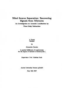
˜ = −1 + 2˜ gs . The corresponding function The score function for the above g˜s , is ψ g ν˜(·) is, as before, a kind of smooth approximation of the absolute value function, with a smoothing parameter of order 1. In order to adapt the algorithm to our purposes, we q 2 use hypothetical density with ν˜(cmk ) = cmk + ζ, and the corresponding score function is q ˜ mk ) = cmk / c2 + ζ. ψ(c mk 2.2 Clustering-based BSS In the case of geometry-based methods, separation of sparse sources can be achieved by clustering along orientations of data concentration in the N-dimensional space wherein each column yk of the matrix Y represents a data point and N is the number of mixtures. Let us consider a two-dimensional noiseless case, wherein two source signals, s1 (t) and s2 (t), are mixed by a 2×2 matrix A, arriving at two mixtures x1 (t) and x2 (t). In this case, the data matrix is constructed from these mixtures x1 (t) and x2 (t)). An example of a scatter plot of 2 mixtures x1 (t) versus x2 (t), constructed from 2 sparse sources, is shown in Figure 1. 3

2

1

0

-1

-2

-3 -3

-2

-1

0

1

2

3

Figure 1: An example of a scatter plot of 2 mixtures x1 (t) versus x2 (t) of 2 sparse sources.

If only one source, say s1 (t), was present, the sensor signals would be x1 (t) = a11 s1 (t) . x2 (t) = a21 s1 (t) All the data points of the scatter diagram x2 versus x1 cluster in this case co-linearly along the straight line defined by the vector [a11 a21 ]T . A similar highly structured distribution results when two sparse natural sources are present simultaneously. An example of fragments of 2 sparse sources is shown in Figure 2. 5


Figure 2: An example of fragments of 2 sparse sources. In this sparse case, at each particular instant where a sample of the first source is large, there is a high probability, that the corresponding sample of the second source is small, and the sampling point projected onto the scatter diagram lies close to the corresponding straight line. The same arguments apply to the complementary points, dominated by the second source. As a result, data points are densely clustered along two dominant orientations, which are directly related to the columns of A. Source signals are rarely sparse in their native original domain. An example of fragments of 2 not sparse sources is shown in Figure 3. An example of a scatter plot of 2 mixtures x1 (t) versus x2 (t), constructed from 2 not sparse sources, is shown in Figure 4.

Figure 3: An example of fragments of 2 not sparse sources. In contrast to the source samples in their original domain, the decomposition coefficients of sources, Eq. (2), are much more sparser. We therefore construct the data matrix Y from the decomposition coefficients of the mixtures, Eq. (3), rather than from the original mixtures. In order to determine orientations of scattered data, we project the data points onto the surface of a unit sphere by normalizing corresponding vectors, and then apply a standard clustering algorithm. This clustering approach is applicable even in cases where the number of sources exceeds the number of sensors. Under such circumstances, separated clusters 6


Figure 4: An example of a scatter plot of 2 mixtures x1 (t) versus x2 (t) of 2 not sparse sources.

consist of samples of scaled versions of sources. An example of scatter plot of 2 mixtures of 6 sparse sources is shown in Figure 5. Note, that in case of natural signals that are not sparse in their native domain (say time, wavelength, position or functions of any other independent variable), a proper projection onto a space of sparse representation will yield a highly structured scatter plot of the decomposition coefficients of the mixtures, similar to the one shown in Figure 5.

Figure 5: An example of scatter plot of 2 mixtures of 6 sparse sources. The proposed clustering procedure used in our BSS algorithm is as follows: 1. Form the feature matrix Y, by inserting samples of the sensor signals or (subset of ) their decomposition coefficients into the corresponding rows of the matrix; 2. Normalize feature vectors: yk = yk /kyk k2 , in order to project data points onto the surface of a unit sphere, where k·k2 denotes the l2 norm;

Before normalization, it is reasonable to remove data points with a very small norm, since these are very likely crosstalk-corrupted by small coefficients from other sources. 7


3. Move data points to a half-sphere, e.g. by forcing the sign of the first coordinate yk1 to be positive: if yk1 < 0 then yk = −yk ;

Without this operation, each set of clustered-along-a-line data points would yield two clusters on opposite sides of the sphere.

4. Estimate cluster centers by using a clustering algorithm. The coordinates of these ˜ centers will form the columns of the estimated mixing matrix A; We used Fuzzy C-means (FCM) clustering algorithm [23] as implemented in the Matlab Fuzzy Logic Toolbox.

2.3 Sources recovery ˆ =A ˆ −1 can be obtained by either clustering, or by the The estimated unmixing matrix W quasi-ML approach, implemented along with the Natural Gradient (we call it simply Natural Gradient), or by other algorithms, which are applied to either the complete data set, or to some subsets of data (see the subsequent section). In any case, this matrix and, therefore, the sources, can be estimated only up to a column permutation and a scaling factor [15]. The sources are recovered in their original domain by ˆ ˆ s(t) = Wx(t). It should be stressed, that if the above clustering approach is used, the estimation of mixing matrix and of sources is not restricted to the case of square mixing matrices, although the sources recovery is more complicated in the rectangular case.

3. Multiscale BSS To provide intuitive insight into the practical implications of our main ideas, we first discuss an example of separation of 1D bloc signals, that are piecewise constant, with random amplitude and duration of each constant piece (Figure 6). 3.1 Motivating example: sparsity of random blocks in the Haar basis space It is well known, that the Haar wavelet basis provides compact representation of block functions. Let take a close look at the Haar wavelet coefficients at different resolution levels j=0,1,...,J. Wavelet basis functions at the finest resolution level j=J are obtained by translation of the Haar mother wavelet:   1 if 0 6 t < 12 −1 if 12 6 t < 1 ϕj=J (t) =  otherwise 0

Taking the scalar product of a function s(t) with the wavelet ϕJ (t − τ ), results in a finite differentiation of the function s(t) at the point t = τ . This implies that the number of non-zero coefficients at the finest resolution for a block function will roughly correspond to the number of jumps of this function. Proceeding to the next, coarser resolution level, we have the wavelet ϕJ−1 (t) = { 12 , if 0 6 t < 1; − 12 , if 1 6 t < 2; 0 otherwise}. The number 8


S1

5

0

-5

100

200

300

400

500

600

700

800

900

1000

100

200

300

400

500

600

700

800

900

1000

100

200

300

400

500

600

700

800

900

1000

100

200

300

400

500

600

700

800

900

1000

S2

5

0

-5

M1

5

0

-5

M2

5

0

-5

Figure 6: Random block signals (two upper) and their mixtures (two lower) of non-zero coefficients at this level still corresponds to the number of jumps, but the total number of coefficients at this level is halved, and so is the sparsity. Proceeding to coarser resolutions, we encounter levels where the support of a wavelet ϕj (t) is comparable to the typical distance between jumps in the function s(t). In this case, most of the coefficients are expected to be nonzero, and, therefore, sparsity fades away. To demonstrate how this influences the accuracy of BSS, we randomly generate two block-signal sources (Figure 6, two upper plots.), and mix them by the crosstalk matrix µ ¶ 0.8321 0.6247 A= . −0.5547 0.7809 Resulting sensor signals, or mixtures, x1 (t) and x2 (t) are shown in the two lower plots of Figure 6. The scatter plot of x1 (t) versus x2 (t) does not exhibit any visible distinct orientation of clustering (Figure 7, left). Similarly, in the scatter plot of all the wavelet coefficients, the two clusters’ orientations are hardly detectable (Figure 7, middle). In contrast, the scatter plot of the wavelet coefficients at the highest level of resolution (Figure 7, right) depicts two distinct orientations, which correspond to the columns of the mixing matrix. Since a cross-talk matrix A is estimated only up to a column permutation and a scaling factor, in order to measure the separation accuracy, we normalize the original sources sm (t) and their corresponding estimated sources s˜m (t). The averaged (over sources) normalized squared error (NSE) is then computed as: NSE =

M ± 1 X (kˆ sm − sm k2 ksm k2 )2 . M m=1

9

(7)


Raw signals

All wavelet coefficients

3

6

3

2

4

2

1

2

1

0

0

-1

-3 -3

0

-1

-2

-2

NG FCM

High resolution WT coefficients

-2

-4

-2

-1

0

1

2

3

10.9 10.2

-6 -6

-4

-2

0

0.056 0.04

2

4

6

-3 -3

-2

-1

0

1

2

3

0.0024 0.002

Figure 7: Separation of mixed block signals: scatter plots of sensor signals (left), and of their wavelet coefficients (middle and right). Lower rows present the normalized mean-squared separation error (%) corresponding to the Natural Gradient (NG), and to the Fuzzy C-Means (FCM) clustering, respectively.

In the noise-free case, this error is equal to the averaged residual cross-talk error (CTE): M 1 X CT E = M m=1

PM

2 ˆ −1 2 ˆ −1 l=1, (A A)ml − (max{(A A)m }) , PM ˆ −1 A)2 ( A ml l=1,

(8)

ˆ −1 A. ˆ −1 A)m } is the largest element in the m-th row of the matrix A where max{(A Resulting separation errors for block sources are presented in the lower part of Figure 7. The largest error (11%) is obtained on the raw data, and the smallest (0.002%) — on the wavelet coefficients at the highest resolution, which have the best sparsity. Using all wavelet coefficients yields intermediate sparsity and performance. 3.2 Multinode representation Our choice of a particular wavelet basis and of the sparsest subset of coefficients was obvious in the above example: it was based on knowledge of the structure of piecewise constant signals. For sources having oscillatory components (like sounds or images with textures), other systems of bases functions, such as wavelet packets [6], [24], trigonometric function libraries [25], or multiwavelets [7] might be more appropriate. In particular, the wavelet packet library consists of the triple-indexed family of functions: ϕj,i,n (t) = 2j/2 ϕn (2j t − i), j, i ∈ Z, n ∈ N,

(9)

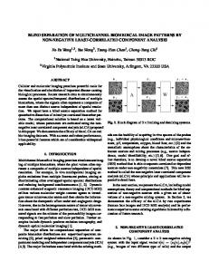
where j, i are the scale and shift parameters, respectively, and n is the frequency-like parameter. [Roughly speaking, n is proportional to the number of oscillations of a mother wavelet ϕn (t)]. These functions form a binary tree whose nodes are indexed by the depth of the level, j, and the node number n = 0, 1, 2, 3, ..., 2j − 1 at the specified level j. The same indexing is applied to corresponding subsets of wavelet packet coefficients (Figure 8), and is used for the scatter diagrams in the section on experimental results. 10


(0,0)

(1,0)

(1,1)

(2,0)

(3,0)

(2,1)

(3,1)

(3,2)

(2,2)

(3,3)

(3,4)

(2,3)

(3,5)

(3,6)

(3,7)

Figure 8: Wavelet Packets tree of subsets of coefficients, indexed by scale (first index) and frequency-like (second index) parameters pair, according to (9)

3.3 Adaptive selection of data subsets for separation As noted, the choice of a particular wavelet basis and of the sparsest subset of coefficients is pretty obvious in the context of the example with block signals. The representations of signals mentioned in the section on the multinode analysis is usually considered in the context of a one-to-one mapping. In particular, in the case of the wavelet packets representation, the best basis is chosen from the library of bases, and is used for a decomposition, providing a complete set of features (coefficients). Another strategy, the basis pursuit [24], chooses the wavelet representation resulting in the smallest l1 -norm of the coefficients. In contrast, in the context of the signal source separation problem, it is useful to extract first an overcomplete set of features. An example of overcomplete set of WP features of mixtures of two Flute signals is presented in Figure 9. In this figure, the tree of scatter plots is formed by the subsets of WP coefficients which ’live’ in the corresponding nodes of the WP tree. The WP analysis reveals an almost noise-free subset of coefficients—the most left scatter plot in the bottom row. This set is best suited for further separation. Generally, in order to construct an overcomplete set of features, our approach to the BSS allows to combine multiple representations (for example, wavelet packets with various generating functions and various families of wavelets, along with DFT, DCT, etc.). After this overcomplete set is constructed, we choose the ’best’ subsets (with respect to some separation criteria) and form a new set used for separation. This set can be either complete or undercomplete. 3.3.1 Heuristic selection of best nodes it is usually difficult to decide in advance which nodes, i.e. subsets of data, contain the sparsest sets of coefficients. Furthermore, there may be a situation wherein only one, or, more generally, not all of the sources are represented in one of the subspaces (at a particular 11


Figure 9: Wavelet Packets (WP) based multinode data structure: the example with mixture of 2 Flutes. Each node depicts scatter plot of WP coefficients of the sensor signals, wherein the coefficients are taken from the corresponding nodes of the WP tree (Figure 8).

node). In this case, the corresponding scatter plot will reveal only one or several dominant orientation. Such a node can still be very useful for separation, provided the points on the scatter plot are well clustered. One can apply the following heuristic approach for choosing the appropriate nodes [26]. First, for every node of the tree, we apply our clustering algorithm, and compute a measure of clusters’ distortion. In our experiments we used a standard global distortion, the mean squared distance of data points to the centers of their own, closest, clusters (here again, the weights of the data points can be incorporated): d=

K X k=1

min k um − yk k2 , m

where K is the number of data points, um is the m-th centroid coordinates, yk is the k-th data point coordinates, and k.k2 is the l2 norm, which is a sum-of-squares distance. Second, we choose a few best nodes with the minimal distortion, combine their coefficients into one data set and apply a separation algorithm, clustering or Natural Gradient, to these data. In the case of the wavelet packets, where two sets of children basis functions span the same subspace as their parent, we should check that there is no redundancy in the set of the best 12


nodes, so that no children and their parents are present at the same time in the final set used for separation. For images, there are four children subsets of functions for each parent set, and therefore, each set of parent coefficients is split into four subsets of coefficients: approximations, horizontal, vertical and diagonal details. Alternatively, the following iterative approach can be used. First, we apply the Wavelet Transform to original data, and apply a standard separation technique to these data in the transform domain. As such separation technique, we can use either the Natural Gradient, our clustering approach, or simply apply some optimization algorithm to minimize the corresponding log-likelihood function. This provides us with an initial estimate of the unmixing matrix W and with the estimated source signals. Then, at each iteration of the algorithm, we apply a multinode representation (for example, WP, or trigonometric library of functions) to the estimated sources, and calculate a measure of sparsity for P each subset |cmk |, its of coefficients. For example, one can consider the l1 norm of the coefficients m,k P log |cmk |, or some other entropy-related measures. modification m,k

Finally, we combine a new data set from the subsets with the highest sparsity (in particular, we can take for example, the best 10% of coefficients), and apply some separation algorithm to the new data. The iteration of the algorithm is completed. This process can be repeated till convergence is achieved. 3.3.2 Error estimator

When signals have a complex nature, the heuristic approach may not be as robust as desired, and the error-related statistical quantities must be estimated. We use the following approach. First, we apply the Wavelet Transform to original data, and apply a standard separation technique (Natural Gradient, clustering, or optimization algorithm to minimize the log-likelihood function) to these data in the transform domain. Second, given the initial estimate of W, and the subsets of data (coefficients of mixtures) for each node, we estimate the corresponding error variance, as described below. Finally, we choose a few best nodes (or, simply, the best one) with small estimated errors, combine their coefficients into one data set, and apply a separation algorithm to these data. In the rest of this section, we focus on the issues related to the estimation of error variance. An estimate of the error covariance matrix can be derived using the second order Taylor expansion of the log-likelihood function. Let W∗ = A−1 be the exact solution of the BSS problem (1); it satisfies h i ˜ W (Y) . W∗ = arg max E L

Further, let Wo be the estimate of W∗ , based on the particular realization of data, Yo , that is, ˜ W (Yo ). Wo = arg max L h i ˜ W (Yo ) 6= 0 (though, E ∇L ˜ W (Y) = 0). We want ˜ Wo (Yo ) = 0, while ∇L Note, that ∇L ∗ ∗ to estimate the error, ∆W = W∗ − Wo . ˜ W (Yo ) around Wo Using the linearization of ∇L ˜ Wo +∆W (Yo ) ' ∇L ˜ Wo (Yo ) + ∇2 L ˜ Wo (Yo ) ∆W ∇L 13


we obtain ˜ W (Yo ) , ∆W ' H−1 ∇L ∗

˜ Wo (Yo ) is the Hessian. Therefore, the error covariance matrix, whose diagwhere H =∇2 L onal elements correspond to the error variances of sources, can be approximated as ¡ £ ¤ ¢T (10) E ∆W∆WT ' H−1 Σ H−1 , where

h i ˜ W (Y)T ˜ W∗ (Y) ∇L Σ = E ∇L ∗

is the covariance matrix of the gradient vector. ˜ k the column stack vector of the k-th data point gradient Further, denote by ∇L ˜ ˜ k )cT )(WT )−1 , ˜ k = ∂ LW (ck ) = (I − ψ(c ∇L k ∂W obtained from (6). Then, since ˜ W (Y) = ∇L

K X k=1

˜k, ∇L

the covariance matrix Σ can be estimated from K data points as: ˆ = K Γ, ˆ Σ where

K h i X ˜ k ∇L ˜ Tk . ˆ= 1 Γ ∇L K k=1

The Hessian matrix can be calculated either analytically, or via numerical evaluation (see [27] for details). In the latter case, its j-th column is approximated by: Hj (w) '

∇L(w+ξej ) − ∇L(w) , ξ

where w is a column stack version of W, ξ is a small constant and ej = [0, 0, ..., 1, 0, ..., 0]T is the vector with the only nonzero entry at the j-th position. The diagonal element ˆε2ii in the error covariance matrix above (10) represents an estimate of the squared error introduced to the reconstructed i-th source by cross-talks from other sources. The analytic expression for the mean square relative contamination of the reconstructed i-th source by the j-th source, for the quasi-ML estimator, is given by [9]: ε2 =

2 2 2 2 2 2 2 1 αi αj (β j /αj + β i − 2β i β j /αj ) , K (1 − αi αj )2 β 2i β 2j

(11)

where K is the number of data samples, and, parameters α and β are dependant on the source-related expectations. In our case, α and β are coefficient-related: ˜ (ci )ci ] ˜ (ci )ci ] E[ψ E[ψ i i q . (12) = ; β αi = 2 ˜ 0 (ci )]E[c2 ] i E[ψ ˜ (ci )]E[c2 ] i i E[ψ i

i

˜ = Note, that the expectation operator E[·] is with respect to the true pdf fC , while ψ(c) 0 ˜ ˜ −(log fC ) is dependent on the hypothetical pdf fC . 14


4. Experiments For reasons given in the previous section, the hypothetical density is used in the expression of q the log-likelihood function (5). In our experiments we use the function ν(cmk , ζ) = c2mk + ζ, as a smooth approximation of the absolute value function.

4.1 Numerical results: theoretic and estimated separation errors In the following experiment, we study the effect of using the quasi log-likelihood instead of the likelihood function on the theoretical error performance. For this purpose, we evaluate expectations in (12) via numerical calculation of the corresponding integrals. Then, for various values of the smoothness parameter ζ, we calculate the error variance according to (11) with the sample size K = 104 , as a function of the true density shape parameter, q ∗ . The results of this calculation are presented in Figure 10. Note, that the error variance drops dramatically as the sparseness of sources increases. This figure shows also that using hypothetical density has a minor effect on the theoretical error.

Figure 10: Theoretical cross-talk error variance: Using the true density, i.e. qth = q ∗ (solid bold line), vs. hypothetical densities with parameters qth = 1, ζ = 0, 10−2 , 10−4 for the ML estimator.

4.1.1 Synthetic exponential sources In the following experiment, we generate two source signals with 104 samples each, drawn from the exponential distribution fs ∼ exp{− |s|q /q} with q ∗ = 0.5. These two signals are mixed together with a 2x2 matrix of normally distributed random numbers. Consequently, 15


the matrix is normalized for the purpose of the error calculation. In order to separate these signals, we apply the following algorithms: 1) the original Natural Gradient with the built-in non-linearity, as implemented in the ICA/EEG Matlab toolbox [22]; 2) the modified Natural Gradient with the non-linearity corresponding to our quasiq log-likelihood −4 function, with parameters qth = 1, and ζ = 10 , that is, using ν(cmk , ζ) = c2mk + 10−4 ; 3) the Matlab function f minu (an implementation of the BFGS Quasi-Newton optimization method [28]), applied to optimize our quasi log-likelihood function with the above parameter values. The following error-related quantities were calculated: 1) the error variance ˆε2 , estimated from data according to (11) by evaluation of corresponding expectations via averaging; 2) the error variances calculated according to (10); these are evaluated for each one of the above three algorithms; 3) actual squared separation errors of the algorithms; 4) theoretical error variance, calculated as described in the beginning of the section 4.1. Tables 1 and 2 summarizes the results of the above experiment; the corresponding values are averaged over the trials. The smallest actual separation error is achieved by using the fminu function. This result is quite expected, since, generally speaking, a batch mode optimization algorithm (such as the BFGS Quasi-Newton) outperforms an online mode optimization algorithm (such as the Natural Gradient). The modified Natural Gradient outperforms the original one, as expected, since its hypothetical pdf is ’closer’ to the true pdf of sources. Also, the error estimate (10) is closer to the theoretical error variance than the estimate according to (11).

Actual sq. error

fminu 8e-5

Mod. NG 1.2e-4

Orig. NG 4.1e-4

Table 1: Actual squared cross-talk errors

Actual sq. error Error var. estimate (11) Error var. estimate (10) Theoretical error variance

fminu 8e-5 1.6e-4 7.8e-5 6.6e-5

Table 2: Estimates of error 4.1.2 Natural sources In the following experiment we apply the fminu function (as described above) to estimate W from each one of 22 data subsets formed by the WP coefficients of mixture of natural images. In Figure 11, we depict the following quantities, for each one of the 22 data subsets: the actual squared separation error and its estimate according to (10). The first subset corresponds to the complete set of the Wavelet Transform (WT) coefficients; the other subsets are indexed on the WP tree. Our ’error predictor’ provides quite accurate estimates of the actual errors. Note, that for the best, the 5-th, subset, the separation error and its estimate are smaller by several orders, as compared to the corresponding quantities of the 1st set, the complete set of the WT coefficients. 16


Figure 11: The actual squared cross-talk error [-], and its estimate (10) [..], evaluated for each one of 22 data sets formed by the corresponding subsets of WP coefficients.

4.2 Separation of simulated and real signals and images The proposed blind separation method based on the wavelet-packet representation, was evaluated by using several types of signals. We have already discussed the relatively simple example of a random block signal. The second type of signal is a frequency modulated (FM) sinusoidal signal. The carrier frequency is modulated by either a sinusoidal function (FM signal) or by random blocks (BFM signal). The third type is a musical recording of flute sounds. Finally, we apply our algorithm to images. An example of such images is presented in Figure 12. Source images and their mixtures are shown at the upper two sets of plots, and the estimated images are shown in the lower two plots. In order to compare accuracy of our multiscale BSS method with that attainable by standard methods, we form the following feature sets: (1) raw data, (2) Short Time Fourier Transform (STFT) coefficients (in the case of 1D signals), (3) Wavelet Transform coefficients (4) Wavelet packet coefficients at the best nodes found by the proposed error estimator (10), while using various wavelet families with different smoothness: Daubechies family - db-1 (or, Haar), db-4, and db-8 mother wavelets. The higher number indicates higher smoothness. In the case of image separation, we used the Discrete Cosine Transform (DCT) instead of the STFT, and the Symmlet (almost symmetric) wavelet family - sym-4 and sym-8 mother wavelets instead of db-4 and db-8, when using wavelet transform and wavelet packets. 4.2.1 Understanding scatter plot and PDF diagrams Let us consider an example of image separation from two mixtures of two sources (Figure 12). Figure 13 shows corresponding scatter plots of the wavelet packet coefficients of mixtures. These scatter plots correspond to the various nodes of the wavelet packet tree. The upper 17


Figure 12: Applying Multiscale BSS method to noise-free mixtures: two source images (upper pair), their mixtures (middle pair) and separated images (lower pair).

Figure 13: Scatter plots of the wavelet packet (WP) coefficients of mixtures of two images; subsets are indexed on the WP tree.

left scatter plot, marked with ’C’, corresponds to the complete set of coefficients at all nodes. The rest are the scatter plots of sets of coefficients indexed on a wavelet packet tree. Generally speaking, the more distinct the two dominant orientations appear on these plots, the more precise is the estimation of the mixing matrix, and, therefore, the better is the quality of separation. Note, that only two nodes (the most left ones in the second from 18


Figure 14: Distributions of angles (orientations) characterizing the scatter diagrams of the WP coefficients of mixtures of two images.

the bottom row) show clear orientations. These nodes will most likely be selected by the algorithm for further estimation process. Figure 14 shows distributions of angles (orientations) formed by points on the corresponding scatter plots of the wavelet packet coefficients at various nodes. Here, the more distinct peaks assure better separation. 4.2.2 Separation from noise-free mixtures Table 3 summarizes results of experiments in which we applied the (original) Natural Gradient to each noise-free feature set. In the case of the WP features, the best subset was selected, using the proposed error estimator (10). In these experiments, we compared the quality of separation of deterministic signals by calculating NSE’s, or residual crosstalk errors, according to (7). In the case of random block and BFM signals, we performed 100 Monte-Carlo simulations and calculated the normalized mean-squared errors (NMSE) for the above feature sets. From Table 3 it is clear that using our best nodes method, implemented with the proposed error estimator, outperforms all other feature sets, including complete set of wavelet coefficients, for each type of signals. Similar improvements were achieved by using the FCM algorithm along with the heuristic data subset selection. In the case of the random block signals, using the Haar wavelet function for the wavelet packet representation yields a better separation than using some smooth wavelet, e. g. ’db-8’. The reason is that these block signals, that are not natural signals, have a sparser representation in the case of the Haar wavelets. In contrast, as expected, natural signals such as the Flute’s signals are better represented by smooth wavelets, that in turn provide a better separation. This is another advantage of using sets of features at multiple nodes along with various families of ’mother’ functions: one can choose best nodes from several decomposition trees simultaneously. 19


Signals Blocks BFM sine FM sine Flutes Images

raw data 10.16 24.51 25.57 1.48 raw data 4.88

STFT 2.669 0.667 0.32 0.287 DCT 3.651

WT db8 0.174 0.665 1.032 0.355 WT sym8 1.164

WT haar 0.037 2.34 6.105 0.852 WT haar 1.114

WP db8 0.073 0.2 0.176 0.154 WP sym8 0.36

WP haar 0.002 0.442 0.284 0.648 WP haar 0.687

Table 3: Normalized squared cross-talk errors [%]: Applying Natural Gradient-based separation to raw data and decomposition coefficients in various domains. In the case of wavelet packets (WP), the best nodes, selected by our error predictor, were used.

4.2.3 Separation from noisy mixtures In order to verify the performance of our method in presence of noise, we added various types of noise (white Gaussian and salt&pepper) to three mixtures of three images at various SNR’s. Table 4 summarizes these experiments in which we applied our approach along with the separation via the modified Natural Gradient algorithm. Signal-to-noise energy ratio Mixtures w. white CT E gaussian noise NSE

100 0.31 0.39

30 0.56 1.69

10 2.05 12.25

3 13.72 54.29

Mixtures with salt&pepper noise

0.32 0.39

1.09 3.11

4.15 16.81

21.69 69.88

CT E NSE

Table 4: Performance of the algorithm in presence of various sources of noise in mixtures: Normalized mean-squared (NSE) and cross-talk (CTE) errors for image separation, applying our multiscale adaptive approach along with the Natural Gradient based separation.

An example of ’difficult’ source separation from noisy mixtures with Gaussian noise is shown in Figure 15. It turns out that the ideas used in wavelet based signal denoising (see for example [29] and references therein), are applied to signal separation from noisy mixtures. In particular, in case of white Gaussian noise, the noise energy is uniformly distributed over all wavelet coefficients at various scales. Therefore, at sufficiently high signal-to-noise energy ratios (SNR), the large coefficients of the signals are only slightly distorted by the noise coefficients. As a result, the presence of noise has a minor effect on the estimation of the unmixing matrix (see the CTE entries in Table 4). Note, that the NSE entries reflect the noise energy passed to the reconstructed sources from the mixtures. Our algorithm provides reasonable separation quality (CT E of about 4%) for SNR’s of about 10 and higher. On the 20


contrast, the Natural Gradient algorithm applied to the noisy mixtures themselves, failed completely to separate source images, arriving at CT E of 47% even in the case of SNR=30. We should stress here that, although our adaptive best nodes method performs reasonably well even in the presence of noise, it is not supposed to further denoise the reconstructed images. The post-filtering can be achieved by some denoising method, after initial source signals are separated. For example, in Figure 15, a simple wavelet denoising method from [29] was applied to separated images.

5. Discussion and Conclusions Although the problem of BSS has been dealt with extensively in the context of linearly mixed signals with no additional effects of the medium such as convolution, one should further extend and improve the state of the art in this research since there are enough important cases where the linear mixing model provides a good approximation of the physics of the problem. This is the case, for example, in the superposition of reflections on an image observed through a semireflective medium [30], [31]. Although the optical system can not be considered in this case to be spatially invariant, and the simple linear mixing model provides only a reasonably good approximation of the problem, the localized multiscale geometrical approach yields excellent results that are by far better than those obtained by the conventional ICA algorithms. One reason for the improvement in this case is that the multinode representation permits ’locking on’ a sparse data subset that can be considered to represent best the result of a locally spatial invariant mixing operation. Examples of (approximately) linear mixing-only in the time domain occur in cross talk between twisted pairs of telephone lines and similarly coupled transmission media. The linear mixing model, without any convolutive effects, provides also a powerful paradigm for the interpretation of a variety of medical signals and images such as optical imaging of normal and malignant tissue, where the signals measured from each group can be considered to reflect mixtures of optical signatures of molecules that are specific to the two groups but at different ratios, as well as of signatures of molecules that are common to both types of tissue. The latter case, to which we devote a great deal of our current effort, represents a problem of unmixing more sources than measured types of signals. Indeed, this type of a problem can not be solved by the ICA or ICA-based algorithms. It can be solved, however, by our approach of clustering of co-linearly scattered data in the space of the coefficients, obtained by projecting the mixtures into the space of sparse representation. The proposed method improves the separation quality by utilizing the structure of signals projected onto a proper space, wherein certain subsets of the wavelet packet coefficients depict significantly better sparsity and, therefore, contribute to better separability than others. Other multiresolution representations based on wavelet-type [5], nonseparable two-dimensional wavelets [7], and multiwindow Gabor-type frames [32] can most likely provide better results in specific cases of image subspaces. The approach depicted in this study using the specific example of wavelet packets can then be adapted to the other representations in a straightforward manner, by constructing the appropriate multinode data structure. In addition, the block partitioning of the image structure into subsets of projected data, can also be incorporated into the proposed multinode framework of BSS, to better exploit the localized spatial-invariant properties of images as well as those of the imag21


Figure 15: Applying Multiscale BSS to noisy mixtures: three source images (1st row), their mixtures (2nd row), the mixtures with additive white Gaussian noise (3d row), separated images (4th row), and post-filtered separated images (5th row)

ing system; properties that are not valid in the case of most signals and images because they are in most cases nonstationary. Nevertheless, the local stationarity is a reasonable assumption in most cases. Of the variety of wavele-type and similar representations that combine the properties of localization, scaling and additional parameters that are specific to each of the representations, there exist an optimal representation for each specific signal 22


or image subspace. Selection or designing of the optimal representation is not, however, a straightforward problem. Although each of the wavelet-type transforms provides a sparse representation of most of the natural signals or images, there major differences in sparsity and clustering in the scatter diagrams can be observed when one uses different representations. In the example of the block signals, it is obvious that Haar wavelets are as close to optimal as one can probably get. Indeed, these wavelets provided much better estimation of the mixing matrix and thereby approximately one fifth of the cross talk error obtained by using smooth (db8) wavelets. The difference between the separation results obtained by using these types of wavelets is further substantiated when the wavelets are casted within the framework of wavelet packets. The squared cross-talk error obtained by using the Haar WP is thirty five times smaller than the error obtained by using the db8-WP, and almost two orders of magnitude smaller than the error obtained by using the conventional (Table 2). If the results obtained in the case of using the Haar-WP for estimation of the mixing matrix and separation of the mixed signals may be considered to be a benchmark, then indeed the match between the natural types of signals and images, used as examples in this study, is far from being optimal. The smallest squared cross-talk error obtained in the case of the separating mixed two flutes’ signals by using the db8-WP is approximately two orders of magnitude larger than the ’benchmark’ result. It is, however, one fourth of error obtained by using the Haar-WP. Thus, whereas the Haar-WP is by far much better than the db8-WP in the case of separating block signals, it is the other way around in the case of flute signals. Indeed the physics of the flute sounds constrains its time varying signals to be smooth, and it is therefore better to use smooth wavelets. Since the structure of images is less understood, it is even more difficult to come up with a recipe for constructing the optimal space of sparse representation. Based on some experience with nonseparable multiwavelets [7], we expect that such representations will provide better (closer to optimal) results. Yet, one has to identify the right mother wavelets that are most suitable for the representation of specific subspaces of images. Simulation results and experiments with mixtures of both one- and two-dimensional natural signals substantiate our assertion that sparsity of the decomposition coefficients has a major effect on quality and efficiency of the BSS. Using the hypothetical log-likelihood function, that is, a smooth approximation of the likelihood derived from the actual pdf of sources, has an insignificant effect on the performance. The estimator of the error variance, based on the Taylor expansion of the quasi log-likelihood function, facilitates efficient selection of the best subset(s) of coefficients and, in fact, provides a reasonable metric for the vaguely defined concept of optimal selection of subsets of coefficients. Once this subset is selected, the mixing matrix is estimated using only this new subset of coefficients, by either clustering approach or by maximizing log-likelihood with some optimization algorithm (e.g., by the Natural Gradient). It should be stressed here that the proposed approach to BSS can be applied in the context of any higher dimensional problem, such as volumetric medical or other natural data, wherein the number of sources is larger than the number of mixtures. In this case, sparse distribution of the properly transformed (projected) mixtures will cluster co-linearly in the higher dimensional scattered data space, and each colinear cluster will serve as an estimator of the elements of one of the source signal. This geometric (clustering) approach 23


simplifies significantly the process of BSS and permits, as noted, the solution of the ill-posed inverse problems in cases that can not be dealt with by the ICA-based approach. Acknowledgments We thank Arkadi Nemirovski for useful discussions. This work has been supported in part by the Ollendorff Minerva Center, by the HASSIP research network program HPRNCT-2002-00285, sponsored by the European Comission, and by the Israeli Ministry of Science. It is currently supported also by the Medical Imaging Group, Dept. of Biomedical Eng. Columbia University and by the ONR-MURI Grant N000M-01-1-0625.

References [1] A. J. Bell and T. J. Sejnowski, “An information-maximization approach to blind separation and blind deconvolution,” Neural Computation, vol. 7, no. 6, pp. 1129—1159, 1995. [2] A. Hyvärinen, “Survey on independent component analysis,” Neural Computing Surveys, no. 2, pp. 94—128, 1999. [3] M. Zibulevsky and B. A. Pearlmutter, "Blind Source Separation by Sparse Decomposition ", Neural Computations 13(4), pp. 863—883, 2001 [4] M. Zibulevsky, B. A. Pearlmutter, P. Bofill, and P. Kisilev, "Blind Source Separation by Sparse Decomposition", chapter in the book: S. J. Roberts, and R.M. Everson eds., Independent Component Analysis: Principles and Practice, Cambridge, 2001. [5] R. R. Coifman and M. V. Wickerhauser. “Entropy-based algorithms for best basis selection”. IEEE Trans. Inform. Theory, 38(2) [6] S. Mallat, A Wavelet Tour of Signal Processing. Academic Press, 1998. [7] D. Stanhill, Y. Y.Zeevi.“2D Multiwavelets for Image Representation”, The 19th Convention of the IEEE, Jerusalem 1996, pp. 251-254 [8] P. Bofill and M. Zibulevsky, Blind separation of more sources than mixtures using the sparsity of the short-time fourier transform, International Workshop on Independent Component Analysis and Blind Signal Separation, (Helsinki, Finland), pp. 87-92, June 2000. [9] D.-T. Pham. Blind separation of instantaneous mixture of sources via an independent component analysis. IEEE Trans. on Sig. Proc., 44(11):2768-2779, Nov. 1996. [10] J.-F. Cardoso. “Infomax and maximum likelihood for blind separation,” IEEE Signal Processing Letters 4 112-114, 1997. [11] B. A. Pearlmutter and L. C. Parra, “A context-sensitive generalization of ICA,” In ICONIP’96, pages 151—157, 1996 24


[12] C. G. Puntonet, A. Prieto, C. Jutten, M. Rodriguez-Alvarez, and J. Ortega, “Separation of sources: A geometry-based procedure for reconstruction of n-valued signals,” Signal Processing, vol. 46, no. 3, pp. 267—284, 1995. [13] A. Prieto, C. G. Puntonet, and B. Prieto, “A neural algorithm for blind separation of sources based on geometric prperties.,” Signal Processing, vol. 64, no. 3, pp. 315—331, 1998. [14] P. Pajunen, A. Hyvärinen, and J. Karhunen, Non-linear blind source separation by self-organizing maps, in ICONIP’96, pp. 1207—1210. [15] P. Comon, C. Jutten, and J. Hérault, “Blind separation of sources, Part II: Statement problem,” Signal Processing, vol. 24, no. 1, pp. 11—20, November 1991. [16] M. S. Lewicki and T. J. Sejnowski, “Learning overcomplete representations,” Neural Computation, 12(2): 337-365, 2000. [17] B. A. Olshausen and D. J. Field “Sparse coding with an overcomplete basis set: A strategy employed by v1? ,” Vision Research, 37:3311—3325, 1997. [18] R. W. Buccigrossi and E. P Simoncelli. Image compression via joint statistical characterization in the wavelet domain. IEEE Trans Image Processing, 8(12):1688-1701, Dec 1999. [19] A. Cichocki, R. Unbehauen, and E. Rummert, “Robust learning algorithm for blind separation of signals,” Electronics Letters, vol. 30, no. 17, pp. 1386—1387, 1994. [20] S. Amari, A. Cichocki, and H. H. Yang, “A new learning algorithm for blind signal separation,” In Advances in Neural Information Processing Systems 8. MIT Press. 1996. [21] J.-F. Cardoso. The equivariant approach to source separation. In Proc. NOLTA, pp. 55-60, 1995. [22] S. Makeig, ICA/EEG toolbox. Computational Neurobiology Laboratory, the Salk Institute. http://www.cnl.salk.edu/˜tewon/ica_cnl.html, 1999. [23] J. C. Bezdek, Pattern Recognition with Fuzzy Objective Function Algorithms. New York: Plenum Press, 1981. [24] Chen, S. C, Donoho, D. L and Sanders, M. A. “Atomic decomposition by basis pursuit,” SIAM J. Sci. Comput., 20, 1, pp. 33-61, 1998. [25] M. V. Wickenhauser “Adapted wavelet analysis: from theory to software,” Wellesley, MA, A K Peters, Ltd., 1994. [26] P. Kisilev, M. Zibulevsky, Y. Y. Zeevi, and B. A. Pearlmutter. “Blind source separation via multinode sparse representation,” In Advances in Neural Information Processing Systems 14. Morgan Kaufmann, 185-191, 2002. 25


[27] P. Kisilev, Y. Y. Zeevi, and M. Zibulevsky. "Subset selection in multiscale blind source separation," CCIT Report no. 512, Technion, June 2002. [28] D. Bertsekas. Nonlinear Programming, 2nd edition, Athena Scientific, 1999. [29] D. L. Donoho, “De-Noising by Soft Thresholding," IEEE Trans. Inf. Theory, vol. 41, 3, pp. 613-627, 1995. [30] H. Farid, and E. H. Adelson, E. H., "Separating reflections from images using independent component analysis", JOSA. Vol. 17, No. 9, pp. 2136-2145, 1999. [31] A. M. Bronstein, M. M. Bronstein, M. Zibulevsky, Y. Y. Zeevi, "Blind Separation of Reflections using Sparse ICA", Proc. 4th International Symposium on Independent Component Analysis, pp.227-232, 2003. [32] M. Zibulski and Y. Y. Zeevi “Discrete Multi-Window Gabor-Type Transforms”, IEEE Trans. on Signal Processing, Vol. 45, No. 6, pp. 1428-1442, 1997.

26