background, still a tremendous number of potentially true statements remain to be ... pressed as simple subject-property-object (s, p, o) triples and are graphically displayed ... represent the truth values of triples that involve the statistical units. Nodes .... can effectively be accessed (in our case the data set given in Table 1).
Multivariate Prediction for Learning on the Semantic Web Yi Huang1 , Volker Tresp1 , Markus Bundschus2 , Achim Rettinger3 , and Hans-Peter Kriegel2 2
1 Siemens AG, Corporate Technology, Munich, Germany Ludwig-Maximilians-Universit¨at M¨unchen, Munich, Germany 3 Karlsruhe Institute of Technology, Karlsruhe, Germany
Abstract. One of the main characteristics of Semantic Web (SW) data is that it is notoriously incomplete: in the same domain a great deal might be known for some entities and almost nothing might be known for others. A popular example is the well known friend-of-a-friend data set where some members document exhaustive private and social information whereas, for privacy concerns and other reasons, almost nothing is known for other members. Although deductive reasoning can be used to complement factual knowledge based on the ontological background, still a tremendous number of potentially true statements remain to be uncovered. The paper is focused on the prediction of potential relationships and attributes by exploiting regularities in the data using statistical relational learning algorithms. We argue that multivariate prediction approaches are most suitable for dealing with the resulting high-dimensional sparse data matrix. Within the statistical framework, the approach scales up to large domains and is able to deal with highly sparse relationship data. A major goal of the presented work is to formulate an inductive learning approach that can be used by people with little machine learning background. We present experimental results using a friend-ofa-friend data set.
1
Introduction
The Semantic Web (SW) is becoming a reality. Most notably is the development around the Linked Open Data (LOD) initiative, where the term Linked Data is used to describe a method of exposing, sharing, and connecting data via dereferenceable Unique Resource Identifiers (URIs) on the Web. Typically, existing data sources are published in the Semantic Web’s Resource Description Framework (RDF), where statements are expressed as simple subject-property-object (s, p, o) triples and are graphically displayed as a directed labeled link between a node representing the subject and a node representing the object (Figure 1). Data sources are interlinked with other data sources in the LOD cloud. In some efforts, subsets of the LOD cloud are retrieved in repositories and some form of logical reasoning is applied to materialize implicit triples. The number of inferred triples is typically on the order of the number of explicit triples. One can certainly assume that there are a huge number of additional true triples which are neither known as facts nor can be derived from reasoning. This might concern both
triples within one of the contributing data sources such as DBpedia4 (intralinks), and triples describing interlinks between the contributing data sources. The goal of the work presented here is to estimate the truth values of triples exploiting patterns in the data. Here we need to take into account the nature of the SW. LOD data is currently dynamically evolving and quite noisy. Thus flexibility and ease of use are preferred properties if compared to highly sophisticated approaches that can only be applied by machine learning experts. Reasonable requirements are as follows: – Machine learning should be “push-button” requiring a minimum of user intervention. – The learning algorithm should scale well with the size of the SW. – The triples and their probabilities, which are predicted using machine learning, should easily be integrated into SPARQL-type querying.5 – Machine learning should be suitable to the data situation on the SW with sparse data (e.g., only a small number of persons are friends) and missing information (e.g., some people don’t reveal private information). Looking at the data situation, there are typically many possible triples associated with an entity (these triples are sometimes called entity molecules or, in our work, statistical unit node set) of which only a small part is known to be true. Due to this large degree of sparsity of the relationship data in the SW, multivariate prediction is appropriate for SW learning. The rows, i.e., data points in the learning matrix are defined by the key entities or statistical units in the sample. The columns are formed by nodes that represent the truth values of triples that involve the statistical units. Nodes representing aggregated information form the inputs. The size of the training data set is under the control of the user by means of sampling. Thereby the data matrix size, and thus also training time, can be made independent or only weakly dependent on the overall size of the SW. For the experiments in this paper we use the friend-of-a-friend (FOAF) data set, which is a distributed social domain describing persons and their relationships in SWformat. Our approach is embedded in a statistical framework requiring the definition of a statistical unit and a population. In our experiments we compare different sampling approaches and analyze generalization on a test set. The paper is organized as follows. In the next section we discuss related work, In Section 3 we discuss how machine learning can be applied to derive probabilistic weights for triples whose truth values are unknown and introduce our approach. In Section 4 we present experimental results using a friend-of-a-friend (FOAF) data set. Finally, Section 5 contains conclusions and outlines further work.
2
Related Work
The work on inductive databases [1] pursues similar goals but is focussed on the lessproblematic data situation in relational databases. In [2] the authors describe SPARQL4 5
http://dbpedia.org/ SPARQL is a new standard for querying RDF-specific information and for displaying querying results.
Fig. 1. Example of an RDF graph displaying a social friendship network in which the income of a person is an attribute. Resources are represented by circular nodes and triples are represented by labeled directed links from subject node to object node. The diamond-shaped nodes stand for random variables which are in state one if the corresponding triples exist. Nodes representing statistical units (here: Persons) have a darker rim.
ML, a framework for adding data mining support to SPARQL. SPARQL-ML was inspired by Microsoft’s Data Mining Extension (DMX). A particular ontology for specifying the machine learning experiment is developed. The SRL methods in [2] are ILP-type approaches based on a closed-world assumption (Relational Bayes Classifier (RBC) and Relational Probabilistic Trees (RPT)). This is in difference to the work presented here, which maintains more of an open-world assumption that is more appropriate in the context of the SW. Another difference is that in our work, both model training and statement prediction can be performed off-line, if desired. In this case inferred triples with their associated certainty values can be stored , e.g., in a triple store, enabling fast query execution. Unsupervised approaches (examples that are suitable for the relational SW domain are [3–6]) are quite flexible and interpretable and provide a probability distribution over a relational domain. Although unsupervised approaches are quite attractive, we fear that the sheer size of the SW and the huge number of potentially true statements make these approaches inappropriate for Web-scale applications. Supervised learning, where a model is trained to make a prediction concerning a single random variable typically shows better predictive performance and better scalability. Typical examples are many ILP approaches [7, 8] and propositionalized ILP approaches [9, 10]. Multivariate prediction generalizes supervised learning to predict several variables jointly, conditioned on some inputs. The improved predictive performance in multivariate prediction, if compared to simple supervised learning, has been attributed to the sharing of statistical strength between the multiple tasks, i.e., data is used more efficiently see [11] and citations therein for a review). Due to the large degree of sparsity of the relationship data in the SW, we expect that multivariate prediction is quite interesting for SW learning and we will apply it in the following.
3
Statistical Modeling
3.1
Defining the Sample
We must be careful in defining the statistical unit, the population, the sampling procedure and the features. A statistical unit is an object of a certain type, e.g., a person. The population is the set of statistical units under consideration. In our framework, a population might be defined as the set of persons that attend a particular university. For learning we use a subset of the population. In the experimental section we will explore various sampling strategies. Based on the sample, a data matrix is generated where the statistical units in the sample define the rows. 3.2
The Random Variables in the Data Matrix
We now introduce for each potential triple a triple node drawn as a diamond-shaped node in Figure 1. A triple node is in state one (true) if the triple is known to exist and is in state zero (false) if the triple is known not to exist. Graphically, one only draws the triple nodes in state one, i.e., the existing triples. We now associate some triples with statistical units. The idea is to assign a triple to a statistical unit if the statistical unit appears in the triple. Let’s consider the statistical unit Jane. Based on the triples she is participating in, we obtain (?personA, typeOf, Person), (Joe, knows, ?personA), and (?personA, hasIncome, High) where ?personA is a variable that represents a statistical unit. The expressions form the random variables (outputs) and define columns in the data matrix.6 By considering the remaining statistical units Jack and Joe we generate the expressions (columns), (?personA, knows, Jane) and (Jack, knows, ?personA). We will not add (Jane, knows, ?personA) since Jane considers no one in the data base to be her friend. We iterate this procedure for all statistical units in the sample and add new expressions (i.e., columns in the data matrix), if necessary. Note that expressions that are not represented in the sample will not be considered. Also, expressions that are rarely true (i.e., for few statistical units) will be removed since no meaningful statistics can be derived from few occurrences. In [12] the triples associated with a statistical unit were denoted as statistical unit node set (SUNS). The matrix formed with the N statistical units as rows and the random variables as columns is denoted as Y . 3.3
Non-random Covariates in the Data Matrix
The columns we have derived so far represent truth values of actual or potential triples. Those triples are treated as random variables in the analysis. If the machine learning algorithm predicts that a triple is very likely, we can enter this triple in the data store. We now add columns that provide additional information for the learning algorithm but which we treat as covariates or fixed inputs. First, we derive simplified relations from the data store. More precisely, we consider the expressions derived in the last subsection and replace constants by variables. For 6
Don’t confuse a random variable representing the truth value of a statement with a variable in a triple, representing an object.
example, from (?personA, knows, Jane) we derive (?personA, knows, ?personB) and count how often this expression is true for a statistical unit ?personA, i.e., we count the number of friends of person ?personA. Second, we consider a simple type of aggregated features from outside a SUNS. Consider first a binary triple (?personA, knows, Jane) . If Jane is part of another binary triple, in the example, (?personA, hasIncome, High) then we form the expression (?personA, knows, ?personB) ∧ (?personB, hasIncome, High) and count how many rich friends a person has. A large number of additional features are possible but so far we restricted ourselves to these two types. The matrix formed with the N statistical units as rows and the additional features as columns is denoted as X. After construction of the data matrix we prune away columns in X and in Y which have ones in fewer than � percent of all rows, where � is usually a very small number. This is because for those features no meaningful statistical analysis is possible. Note that by applying this pruning procedure we reduce the exponential number of random variables to typically a much smaller set. 3.4
Algorithms for Learning with Statistical Units Node Sets
In a statistical setting as described above, the statistical unit node set (SUNS) is defined mostly based on local neighborhoods of statistical units. By adding aggregated information derived from the neighborhood, homophily can also be modeled. For instance, the income of a person can be predicted by the average income of this person’s friends. As we will see in the experiments, the resulting data matrices are typically highdimensional and sparse. In this situation, multivariate prediction approaches have been most successful [11]. In multivariate prediction all outputs are jointly predicted such that statistical strength can be shared between outputs. The reason is that some or all model parameters are sensitive to all outputs, improving the estimates of those parameters.7 We apply four different multivariate prediction approaches. First, we utilize a reduced rank penalized regression (RRPP) algorithm to obtain an estimated matrix via the formula � � dk UrT Y Yˆ = Ur diagr dk + λ where dk and Ur are derived from a r-rank eigen decomposition of the kernel� matrix � k K ≈ Ur Dr UrT . Ur is a N × r matrix with r orthonormal columns, diagr dkd+λ is a diagonal matrix containing the r largest eigen values and λ is a regularization parameter. The kernel matrix K can be defined application specifically. Typically, as in the following application, one works with a linear kernel defined by K = ZZ T , where Z = [αX, Y ] is formed by concatenating X and Y and where α is a positive weighting factor.8 7
8
Although the completion is applied to the entire matrix, only zeros —representing triples with unknown truth values— are overwritten. Alternatively, we can define a linear kernel solely based on the input attributes K = XX T , when α → ∞, or solely based on the output attributes K = Y Y T , when α = 0.
Fig. 2. Entity-relationship diagram of the LJ-FOAF domain
Besides RRPP we investigate three other multivariate prediction approaches based on matrix completion, i.e., singular value decomposition (SVD), non-negative matrix factorization (NNMF) [13] and latent Dirichlet allocation (LDA) [14]. All approaches estimate unknown matrix entries via a low-rank matrix approximation. NNMF is a decomposition under the constraints that all terms in the factoring matrices are nonnegative. LDA is based on a Bayesian treatment of a generative topic model. After matrix completion of the zero entries in the data matrix, the entries are interpreted as certainty values that the corresponding triples are true. After training, the models can also be applied to statistical units in the population outside the sample.
4
Experiments
4.1
Data Set and Experimental Setup
Data Set: The experiments are based on friend-of-a-friend (FOAF) data. The purpose of the FOAF project [15] is to create a web of machine-readable pages describing people, their relationships, and people’s activities and interests, using W3C’s RDF technology. The FOAF ontology is based on RDFS/OWL and is formally specified in the FOAF Vocabulary Specification 0.919 . We gathered our FOAF data set from user profiles of the community website LiveJournal.com10 . All extracted entities and relations are shown in Figure 2. In total we collected 32,062 persons and all related attributes. An initial pruning step removed little connected persons and rare attributes. Table 1 lists the number of different individuals (top rows) and their known instantiated relations (bottom rows) in the full triple set, in the pruned triple set and in triples sets in different experiment settings (explained below). The resulting data matrix, after pruning, has 14,425 rows (persons) and 15,206 columns. Among those columns 14,425 ones (friendship attributes) refer to the property knows. The remaining 781 columns (general attributes) refer to general information 9 10
http://xmlns.com/foaf/spec/ http://www.livejournal.com/bots/
setting 1
setting 2
setting 3
setting 4
Fig. 3. Evaluated sampling strategies
about age, location, number of blog posts, attended school, online chat account and interest. Data Retrieval and Sampling Strategies: In our experiments we evaluated the generalization capabilities of the learning algorithms given eight different settings. The first four settings are illustrated in Figure 3. A cloud symbolizes the part of the Web that can effectively be accessed (in our case the data set given in Table 1). Crosses represent persons that are known during the training phase (training set) and circles represent persons with knows relations that need to be predicted. Setting 1 describes the situation where the depicted part of the SW is randomly accessible, meaning that all instances can be queried directly from triple stores. Statistical units in the sample for training are randomly sampled and statements for other randomly selected statistical units are predicted for testing (inductive setting). In this setting, persons are rarely connected by the knows relations. The knows relation in the training and test set is very sparse (0.18%). Setting 2 also shows the situation where statistical units in the sample are randomly selected, but this time the truth values of statements concerning the statistical units in the training sample are predicted (transductive setting). Some instances of the knows relation of the selected statistical units are withheld from training and used for prediction. Prediction should be easier here since the statistics for training and prediction match perfectly. Setting 3 assumes that the Web address of one user (i.e., one statistical unit) is known. Starting from this random user, users connected by the knows relation are gathered by breadth-first crawling and are then added as rows in the training set. The test set is gathered by continued crawling (inductive setting). In this way all profiles are (not necessarily directly) connected and training profiles show a higher connectivity (1.02%) compared to test profiles (0.44%). In this situation generalization can be expected to be easier than in setting 1 and 2 since local properties are more consistent than global ones. Setting 4 is the combination of settings 2 and 3. The truth values of statements concerning the statistical units in the training sample are predicted (transductive setting). Instances of the knows relation are withheld from training and used for prediction. Settings 5-8 use the same set of statistical units as settings 1-4 respectively. The difference is that in settings 1-4 the data matrix only contains friendship relations
to persons in the sample whereas in settings 5-8, the data matrix contains friendship relations any persons in the population. In settings 5-8 we remove those users (friendship attributes) who are known by less than ten users (statistical units), i.e., � = 10. We ended up with a large number of ones in the data matrix when compared to settings 1-4. The concrete numbers of the statistical units and the friendship attributes are shown in Person (row) and Person (col) respectively in Table 1. Evaluation Procedure and Evaluation Measure: The task is to predict potential friends of a person, i.e., knows statements. For each person in the data set, we randomly selected one knows friendship statement and set the corresponding matrix entry to zero, to be treated as unknown (test statement). In the test phase we then predicted all unknown friendship entries, including the entry for the test statement. The test statement should obtain a high likelihood value, if compared to the other unknown friendship entries. Here we use the normalized discounted cumulative gain (NDCG) [16] (described in the Appendix) to evaluate a predicted ranking. Benchmark methods: Baseline: Here, we create a random ranking for all unknown triples, i.e., every unknown triple gets a random probability assigned. Friends of friends in second depth (FOF, d=2): We assume that friends of friends of a particular person might be friends of that person too. From the RDF graph point of view the knows relation propagates one step further alongside the existing knows linkages. 4.2
Results
In settings 1 and 2 we randomly sampled 2,000 persons for the training set. In addition, in setting 1 we further randomly sampled 2,000 persons for the test set. In setting 3, 4,000 persons were sampled, where the first half was used for training and the second half for testing. Setting 4 only required the 2,000 persons in the training set. In settings 5-8 we followed the same sampling strategies as in settings 1-4 respectively and extracted all users known by the sampled users to form the friendship attributes. In each case, sampling was repeated 5 times such that error bars could be derived. Table 1 reports details of the samples (training set and, if applicable, test set). The two benchmark methods and the four multivariate prediction approaches proposed in Section 3.4 were then applied to the training set. For each sample we repeated the evaluation procedure as described above 10 times. Since NNMF is only applicable in a transductive setting, it was only applied in setting 1, 3, 5 and 7. Moreover, the FOF, d=2 is not applicable in settings 5-8, since it is impossible for many statistical units to access the friends of their friends. Figures 4 and 5 show the experimental results for our FOAF data set. The error bars show the 95% confidence intervals based on the standard error of the mean over the samples. The figures plot the NDCG all score of the algorithms against the number of latent variables in settings 1, 2, 5, 6 in Figure 4 and in settings 3, 4, 7, 8 in Figure 5. The best NDCG all scores of all algorithms in different settings are shown in Table 2, where r indicates the number of latent variables achieving the best scores.
2,000 2,000 2,000 2,000 2,000 2,000 320 320 320 329 329 329 118 118 118 5 5 5 4 4 4 5 5 5 7,339 40,786 17,613 0.18% 1.02% 0.44% 1,106 1,172 1,217 747 718 749 246 216 208 1,087 1,168 1,075 715 779 784 1,992 1,994 1,991
setting 1 setting 2 setting 3 training test training test
32,062 14,425 2,000 2,000 - 2,000 2,000 5,673 320 320 320 15,744 329 329 329 4,695 118 118 118 5 5 5 5 4 4 4 4 5 5 5 5 530,831 386,327 7,311 7,339 0.05% 0.19% 0.18% 0.18% 24,368 7,964 1,122 1,106 31,507 5,088 676 747 9,616 1,659 206 246 19,021 8,319 1,134 1,087 10,040 5,287 777 715 31,959 14,369 1,993 1,992
pruned
setting 5 training test
2,000 2,000 2,000 2,000 1,122 1,122 320 320 320 329 329 329 118 118 118 5 5 5 4 4 4 5 5 5 40,786 14,909 16,869 1.02% 0.66% 0.75% 1,172 1,122 1,106 718 676 747 216 206 246 1,168 1,134 1,087 779 777 715 1,994 1,993 1,992
setting 4
setting 7 training test
2,000 2,000 2,000 1,122 1,297 1,297 320 320 320 329 329 329 118 118 118 5 5 5 4 4 4 5 5 5 16,869 41,705 18,595 0.75% 1.61% 0.72% 1,106 1,172 1,217 747 718 749 246 216 208 1,087 1,168 1,075 715 779 784 1,992 1,994 1,991
setting 6 2,000 1,297 320 329 118 5 4 5 41,705 1.61% 1,172 718 216 1,168 779 1,994
setting 8
setting 1
setting 2
setting 4
0.1094 ± 0.0001 0.1094 ± 0.0001 0.1495 ± 0.0077 0.1495 ± 0.0077 NaN 0.2983 ± 0.0197 r=150 0.2085 ± 0.0147 0.3027 ± 0.0179 r=200 r=100 0.2288 ± 0.0123 0.3374 ± 0.0117 r=200 r=200 0.2252 ± 0.0049 0.3315 ± 0.0109 r=400 r=400
setting 3
setting 6 0.1213 ± 0.0005 0.1213 ± 0.0005 NaN NaN NaN 0.2864 ± 0.0067 r=150 0.2688 ± 0.0044 0.3176 ± 0.0092 r=150 r=150 0.2640 ± 0.0022 0.3359 ± 0.0079 r=150 r=200 0.2956 ± 0.0019 0.3582 ± 0.0049 r=400 r=400
setting 5
setting 8 0.1216 ± 0.0042 0.1216 ± 0.0042 NaN NaN NaN 0.3217 ± 0.0403 r=100 0.2407 ± 0.0413 0.3411 ± 0.0179 r=100 r=50 0.2331 ± 0.0143 0.3470 ± 0.0372 r=150 r=200 0.2607 ± 0.0088 0.3591 ± 0.0237 r=400 r=400
setting 7
Table 2. Best NDCG all averaged over samples with 95% confidence interval where r stands for the number of latent variables
Baseline 0.1092 ± 0.0003 0.1092 ± 0.0003 F OF, d = 2 0.2146 ± 0.0095 0.2146 ± 0.0095 NNMF NaN 0.2021 ± 0.0058 r=100 SV D 0.2174 ± 0.0061 0.2325 ± 0.0074 r=150 r=100 LDA 0.2514 ± 0.0049 0.2988 ± 0.0057 r=200 r=200 RRP P 0.2483 ± 0.0018 0.2749 ± 0.0037 r=400 r=400
Method
Table 1. Number of individuals and number of instantiated relations in the full triple set, in the pruned triple set (see text) and statistics for the different experimental settings
Concept P erson (row) #Indivi. P erson (col) Location School Interest On.ChatAcc. Date #BlogP osts Role knows #Inst. (sparsity) residence attends has holds dateOf Birth posted
full
(a)
(c)
(b)
(d)
Fig. 4. Comparison between different algorithms. NDCG all is plotted against the number of latent variables: (a)-(d) for settings 1, 2, 5, 6 respectively.
First, we observe that the experimental results in settings 5-8 are much better than those in settings 1-4. This can be attributed to the fact that in settings 5-8 columns were pruned more drastically and a more dense friendship pattern was achieved. Another observation is that all four multivariate prediction approaches clearly outperform the benchmark algorithms in all settings, although in settings 1 and 2 NNMF and SVD are only slightly better than FOF, d=2. Furthermore, we observe that LDA and RRPP outperform NNMF and SVD in each setting, and that LDA and RRPP are not sensitive to the number of latent variables as long as the chosen number is reasonably high. LDA reaches its maximum NDCG score, for instance, with r = 150 latent variables in setting 4 and the performance does not deteriorate when the number of latent factors is increased. The score of RRPP keeps increasing and does not drop down in the observed range of the number of latent variables. In contrast, NNMF and SVD are sensitive with respect to the predefined number of latent variables. Comparing the results over different settings we can observe that for the multivariate prediction approaches one obtains best performance in setting 4, next best performance
(a)
(c)
(b)
(d)
Fig. 5. Continue Figure 4: (a)-(d) for settings 3, 4, 7, 8 respectively.
in setting 2, then follows setting 1 and 3 is the most difficult setting. The corresponding order can be seen in settings 5-8. The baseline method, random guess, is independent to the settings and achieves almost the same score in all settings. The fact that the scores in settings 4 and 8 are the best indicates that a link-following sampling strategy in general gives better performance than random sampling. Similar results in statistical comparisons between random and link-following sampling have been obtained in other works, e.g., [17]. Finally, we observe that the prediction performance in setting 1 is only slightly worse than the prediction performance in setting 2, while the prediction performance in setting 4 is much better than in setting 3. This phenomenon occurs in settings 5-8 too. We attribute this to the general statistics in the training and the test set which are very different both in setting 3 and setting 7. In Table 1 it is apparent that for instance, in setting 3 the knows relation in the training data set (1.02%) is significantly more dense than in the test data set (0.44%). Intuitively speaking, the people in the training know each other quite well, but the people in the test do not know the people in the training as much.
5
Conclusions and Outlook
The paper describes extensions to the SUNS approach introduced in [12]. The SUNS approach is based on multivariate prediction which is quite suitable for the typical SW data situation. In our experiments based on the FOAF data set, LDA and RRPP showed best performance, and the performance is insensitive to the rank of the approximation, resp. to the number of latent variables. This can be explained by the fact that LDA, in contrast to NNMF, is a Bayesian approach and by the fact that the RRPP, in contrast to SVD, is regularized. Thus LDA or RRPP can be default methods being insensitive to exact parameter tuning. All four approaches exploited the benefits of multivariate prediction since approaches based on single predictions (not reported here) did not even reach the performance of the benchmark approaches. The proposed approach can be extended in many ways. One might want to allow the user to specify additional parameters in the learning process, if desired, along the line of the extensions described in [2]. Another extension concerns ontological background knowledge. So far, ontological background knowledge was considered by including logically inferred statements into learning. Ongoing work explores additional ways of exploiting ontological background information, e.g., for structuring the learning matrix. Finally we want to demonstrate how learned probabilistic statements can be queried. The following SPARQL query illustrates a query for LiveJournal users who live in Munich and might want to be Trelena’s friend: 1 2 3 4 5 6 7 8 9 10 11
PREFIX ya: http://blogs.yandex.ru/schema/foaf/ PREFIX foaf: http://xmlns.com/foaf/0.1/ PREFIX dc: http://purl.org/dc/elements/1.1/ SELECT DISTINCT ?person WHERE { ?person ya:located ?city . ?person foaf:knows WITH PROB ?prob . FILTER REGEX(?city, "Munich") . } ORDER BY DESC(?prob)
The query includes the predicted knows triples for Trelena and rates them by predicted probability. Acknowledgements: We acknowledge funding by the German Federal Ministry of Economy and Technology (BMWi) under the THESEUS project and by the EU FP 7 Large-Scale Integrating Project LarKC.
6
Appendix
Details on the NDCG Score We use the normalized discounted cumulative gain (NDCG) to evaluate a predicted ranking. NDCG is calculated by summing over all the gains in the rank list R with a log
discount factor as NDCG(R) =
1 X 2r(k) − 1 , Z log(1 + k) k
where r(k) denotes the target label for the k-th ranked item in R, and r is chosen such that a perfect ranking obtains value 1. To focus more on the top-ranked items, we also consider the NDCG@n which only counts the top n items in the rank list. These scores are averaged over all ranking lists for comparison.
References 1. Raedt, L.D., Jaeger, M., Lee, S.D., Mannila, H.: A theory of inductive query answering. In: ICDM. (2002) 2. Kiefer, C., Bernstein, A., Locher, A.: Adding data mining support to sparql via statistical relational learning methods. In: ESWC 2008, Springer-Verlag (2008) 3. Getoor, L., Friedman, N., Koller, D., Pferrer, A., Taskar, B.: Probabilistic relational models. In Getoor, L., Taskar, B., eds.: Introduction to Statistical Relational Learning. MIT Press (2007) 4. Domingos, P., Richardson, M.: Markov logic: A unifying framework for statistical relational learning. In Getoor, L., Taskar, B., eds.: Introduction to Statistical Relational Learning. MIT Press (2007) 5. Xu, Z., Tresp, V., Yu, K., Kriegel, H.P.: Infinite hidden relational models. In: Uncertainty in Artificial Intelligence (UAI). (2006) 6. Kemp, C., Tenenbaum, J.B., Griffiths, T.L., Yamada, T., Ueda, N.: Learning systems of concepts with an infinite relational model. In: Poceedings of the National Conference on Artificial Intelligence (AAAI). (2006) 7. Quinlan, J.R.: Learning logical definitions from relations. Machine Learning 5(3) (1990) 8. Muggleton, S., Feng, C.: Efficient induction of logic programs. In: Proceedings of the 1st Conference on Algorithmic Learning Theory, Ohmsma, Tokyo (1990) 9. De Raedt, L.: Attribute-value learning versus inductive logic programming: The missing links (extended abstract). In: ILP ’98: Proceedings of the 8th International Workshop on Inductive Logic Programming, Springer-Verlag (1998) 10. Lavraˇc, N., Dˇzeroski, S., Grobelnik, M.: Learning nonrecursive definitions of relations with LINUS. In: EWSL-91: Proceedings of the European working session on learning on Machine learning. (1991) 11. Tresp, V., Yu, K.: Learning with dependencies between several response variables. In: Tutorial at ICML 2009. (2009) 12. Tresp, V., Huang, Y., Bundschus, M., Rettinger, A.: Materializing and querying learned knowledge. In: Proceedings of the First ESWC Workshop on Inductive Reasoning and Machine Learning on the Semantic Web. (2009) 13. Lee, D.D., Seung, H.S.: Learning the parts of objects by non-negative matrix factorization. Nature (1999) 14. Blei, D.M., Ng, A.Y., Jordan, M.I.: Latent dirichlet allocation. J. Mach. Learn. Res. 3 (2003) 15. Brickley, D., Miller, L.: The Friend of a Friend (FOAF) project, http://www.foaf-project.org/ 16. Jarvelin, K., Kekalainen, J.: IR evaluation methods for retrieving highly relevant documents. In: SIGIR’00. (2000) 17. Neville, J., Gallagher, B., Eliassi-Rad, T.: Evaluating statistical tests for within-network classifiers of relational data. In: ICDM 2009. (2009)