Multiyear Discrete Stochastic Programming with a Fuzzy Semi-Markov

Applied Mathematics, 2016, 7, 482-495 Published Online March 2016 in SciRes. http://www.scirp.org/journal/am http://dx.doi.org/10.4236/am.2016.76044

Multiyear Discrete Stochastic Programming with a Fuzzy Semi-Markov Process C. S. Kim1, Richard M. Adams2, Dannele E. Peck3 1

Economic Research Service, U.S. Department of Agriculture, Washington, DC, USA Department of Applied Economics, Oregon State University, Corvallis, OR, USA 3 Department of Agricultural and Applied Economics, University of Wyoming, Laramie, WY, USA 2

Received 20 October 2016; accepted 21 March 2016; published 24 March 2016 Copyright © 2016 by authors and Scientific Research Publishing Inc. This work is licensed under the Creative Commons Attribution International License (CC BY). http://creativecommons.org/licenses/by/4.0/

Abstract Drought conditions at a given location evolve randomly through time and are typically characterized by severity and duration. Researchers interested in modeling the economic effects of drought on agriculture or other water users often capture the stochastic nature of drought and its conditions via multiyear, stochastic economic models. Three major sources of uncertainty in application of a multiyear discrete stochastic model to evaluate user preparedness and response to drought are: (1) the assumption of independence of yearly weather conditions, (2) linguistic vagueness in the definition of drought itself, and (3) the duration of drought. One means of addressing these uncertainties is to re-cast drought as a stochastic, multiyear process using a “fuzzy” semi-Markov process. In this paper, we review “crisp” versus “fuzzy” representations of drought and show how fuzzy semi-Markov processes can aid researchers in developing more robust multiyear, discrete stochastic models.

Keywords Drought, Discrete Stochastic Economic Modeling, Fuzzy Logic, Fuzzy Markov Process, Fuzzy Semi-Markov Process

1. Introduction The impacts of drought on water supplies and those dependent on such supplies have long been an important topic for economists and policy makers. Climate projections for key hydrologic inputs—seasonal precipitation, snowpack storage, evaporative loss, and frequency and severity of drought—are used to anticipate future stresses on water quantity and variability. Water managers use these projections to allocate seasonal water sup-

How to cite this paper: Kim, C.S., Adams, R.M. and Peck, D.E. (2016) Multiyear Discrete Stochastic Programming with a Fuzzy Semi-Markov Process. Applied Mathematics, 7, 482-495. http://dx.doi.org/10.4236/am.2016.76044

C. S. Kim et al.

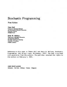
plies across various classes of users. For example, public irrigation districts in the western U.S. typically issue water allocation declarations in March, based on hydrologic forecasts, to help irrigators plan for the coming irrigation season. In periods of sharply reduced water supplies, such as recent multiyear droughts in California (Figure 1), such allocation decisions must reflect a range of competing demands, including in stream flow requirements to protect associated species and ecosystems. Discrete stochastic programming (DSP) has been widely used as an optimization method to assess the benefits and costs of alternative water allocation decisions during varying degrees of drought [1]-[3]. DSP is a useful technique based on traditional probability theory. To illustrate water supply uncertainty in a discrete stochastic programming framework, first consider the following single-year linear programming model: Max Z = c′x ,

(1.1)

subject to: Ax ≤ b

(1.2)

where x = (xj) is a vector of control variables with x ≥ 0, c = (cj) is an (n × 1) column vector of constants, A = (aij)

2000

2002

2004

2006

2008

2010

2012

2014

Figure 1. Severity and duration of drought in California (Source: The National Drought Mitigation Center—USDA).

483

C. S. Kim et al.

is an (m × n) matrix of constants, and b = (bi) is an (m × 1) column vector of constants. The corresponding discrete stochastic linear programming problem, first proposed by Cocks [4], introduces uncertainty into one or more model parameters, such that they satisfy the conditions of a probability distribution:

P ( A= , b, c )

, ck )  ( Ak , bk=

P= ( k 1, 2, , K ) , k

(1.3)

K

where

∑ Pk = 1 . k =1

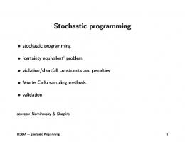
Most previous studies that use DSP to address uncertainty caused by randomness of hydrologic inputs assume a small number of discrete states of nature, sometimes just a binary set (e.g., “drought” = 24 acre-inches of water; “normal” = 40 acre-inches, as in Figure 2). This type of linguistic vagueness of the term “drought” can be illustrated by considering the Palmer Drought Severity Index (PDSI), employed by the National Oceanic and Atmospheric Administration (NOAA) to communicate drought conditions to the public. The PDSI comprises five states of drought, including mild, moderate, severe, extreme, and exceptional. Each state of drought comprises a range of temperature and precipitation conditions. The same quantity of precipitation may therefore result in different states of drought, depending on temperature conditions. A given water allotment does not always result in the same state of drought; instead, it has the potential to lead to various states of drought (i.e., it has “grades of membership” in different states of drought). Which state of drought should actually be assigned to a given water allotment (or vice versa) depends on many other complex factors, including but not limited to temperature, available water content of the soil, and other conditions not easily incorporated into an economic model. Correct assignment of a state of drought is important because severe, extreme, or exceptional drought implies a significant reduction in crop production, whereas mild or moderate drought implies a much smaller reduction. An inadequate number of states of nature in a programming model may produce management recommendations that are not robust when they are applied to a real-world setting that has numerous states of nature (e.g., a continuum of water allocations) [5]. There is another linguistic vagueness in the definition of “drought”, specifically when modelers attempt to assign this term to a specific quantity of irrigation water (e.g., “drought” = 24 acre-inches of water, not 20 or 26, but exactly 24). In addition to linguistic vagueness, the agricultural economics literature has rarely discussed uncertainty about the duration of drought. Peck and Adams [3] developed a multiyear, discrete stochastic model of irrigation water use on a multi-crop farm that faces uncertain surface-water supplies due to the possibility of drought. They then used the model to identify optimal drought preparedness and response plans and measure associated economic benefits that result as the severity and duration of drought is revealed over a six-year period. While they confirmed that the effects of two consecutive years of drought are greater than the sum of two single-year (non-consecutive) droughts, due to inter-annual crop-rotation constraints, they assumed just two discrete (i.e., crisply-defined) states of nature (“normal” = 40 acre-inches per acre; “dry” = 24 acre-inches per acre) and also assumed independence between individual years’ states of nature (i.e., the occurrence of drought in one year did not change the probability of drought in subsequent years). They left more sophisticated approaches to these

(1 − Pk)

Pk

0

24

40

Figure 2. Probabilistic crisp bounds for water allotments.

484

Water allotment (acre inches)

C. S. Kim et al.

three modeling issues—linguistic vagueness, assumption of independence of yearly water allocation, and more complex assumptions about uncertainty of drought duration—for future research. Uncertainty caused by linguistic vagueness has been dealt with more recently using fuzzy logics [6]. A principal difference between discrete-stochastic and fuzzy optimization approaches is in the way uncertainty is modeled: discrete stochastic programming represents random parameters through discrete or continuous probability functions, whereas fuzzy programming treats random parameters as fuzzy numbers and hence constraints as fuzzy sets [7]. Fuzzy programming can be classified into two types.1 Possibilistic fuzzy programming considers uncertainties in the objective function coefficients, c, in Equation (1.1), as well as in the constraint coefficients, A and b, in Equation (1.2). Flexible fuzzy programming considers uncertainties associated only with right-hand-side constraints, b [8]-[10]. Furthermore, discrete stochastic programming requires the constraints to be exactly satisfied in each state of nature. For example, the model cannot choose a crop plan that consumes more than the exact quantity of water (24 or 40 acre-inches) that is ultimately revealed to be available. The most commonly used fuzzy mathematical programming method for this type of linguistic vagueness is to transform a crisp programming model into a series of crisp programming problems [11]. Meanwhile, the second type of linguistic vagueness has been dealt with using interval fuzzy programming approaches [12]. However, there are a few shortcomings of fuzzy programming. For example, although it can be used to evaluate the economic effects of drought severity, it is not capable of dealing with randomness in the duration of drought (or other random phenomena) [13]. To overcome the shortcomings of the discrete stochastic programming approach [including: (1) crisp definitions for each state of nature, (2) assumed independence of states of nature across multiple periods, e.g., if the probability of drought in a single year is 1/3, then the probability of a two-year drought is simply 1/3 × 1/3 or 1/9), and (3) inability to accommodate uncertainty about future states of nature, i.e., uncertainty about drought duration], we first provide in Section 2 a definition of drought, and then discuss uncertainty caused by linguistic vagueness in the term “drought”. We also introduce readers to fuzzy logic for drought severity, where a continuous range of possible water quantities are assigned various grades of membership in a set of drought severity. In section 3, we introduce a semi-Markov process, which allows more complex assumptions about both the probability (or possibility) of transitioning from one state of nature to the next (e.g., the conditional probability (or possibility) of drought occurring next year, given drought occurred this year, is not necessarily equal to the unconditional probability of drought in a single year), and the duration between two transitions. Fuzzy logic and semi-Markov processes are then combined into a fuzzy semi-Markov process, which enables us to capture uncertainty in both drought severity and duration simultaneously. This fuzzy semi-Markov process can ultimately be incorporated in a discrete stochastic programming framework to overcome the shortcomings mentioned earlier. Finally, in Section 4, we present numerical examples of conditional possibility of drought duration, given a specific state of drought severity. These numerical examples highlight potential implications of using fuzzy semi-Markov processes rather than traditional probability-based representations of multiyear drought.

2. Linguistic Vagueness and Fuzzy Logic To evaluate the impacts of drought conditions and associated preparedness and response plans, a clear definition of drought must be provided. One definition of drought is the case in which irrigation water supplied is less than irrigation water demanded, due to inadequate rainfall, snow pack, or other weather conditions. As the difference between irrigation water demanded and supplied increases, severity of drought intensifies along a continuous gradient. While the characterization of drought varies across studies, the following definition of drought provided by Yevjevich [14] has been widely used [6] [15] [16]:

0 if Si < S0 yi =  1 if Si ≥ S0

1, 2, 3,) (i =

,

(2.1)

where S0 is a constant water allotment threshold (such as 40 acre-inches Peck and Adams [3] used for water allotment under normal weather condition) and Si is the ith severity state. A Bernoulli variable yi plays a 1

Both possibilistic and flexible fuzzy programming can be presented in interval fuzzy programming [12].

485

C. S. Kim et al.

significant role in estimation of the holding time (i.e., duration) probability mass function of drought in later section of semi-Markov chains. When economic models represent drought in binary terms (i.e., a water allocation either qualifies or does not qualify as drought), this overly-simplified or deceivingly-crisp (as opposed to fuzzy) measurement of drought severity can cause inefficient resource allocation. Unlike this crisp set (in which an element is either a member of the set or not), fuzzy sets allow elements to be included through a degree of membership, as expressed by a membership function, thus relaxing the binary state assumption [6] [17]. Introduced by Zadeh [18], fuzzy logic and fuzzy set theory have since been widely adopted to deal with linguistic vagueness in various mathematical optimization models, including fuzzy dynamic programming [19] [20], and optimal fuzzy control [21]. Every fuzzy set is associated with a membership function, a curve that defines how each point in the universe of discourse maps to a membership value (or degree of membership) between 0 and 1. Membership functions are often assumed to be piece-wise linear and triangular or trapezoidal in shape [8], or nonlinear such as a sigmoid membership function [15]. The following is a technical definition of a fuzzy set and membership function in the context of drought. Definition 1. Let W = w1 , w2 , , wn be the universe of discourse, where wi is the ith possible value that a future water allocation could take. A fuzzy set, S, in a nonempty set, W, is a set of ordered pairs, = S ( w, f s ( w) ) , w ∈ W , where fs(w) is called the membership function or grade of membership of w in S, which takes on a real number in the interval [0, 1]. Because different water allocations wi ( i = 1, 2,) lead to different levels of drought-severity, Si, many Si exist. Collectively, these Si are a fuzzy subset of a set S, which is defined as a set of ordered pairs, ( wi , f S ( wi ) ) , where f S ( wi ) is the grade of membership of wi in S. The set S represents all water allotment levels, including a particular drought-severity category, such as mild. Fuzzy set theory allows us to define mild drought as a range of possible water deficits, each with its own grade of membership in the set (with its grade falling anywhere between 0 and 1, as described in Equation (2.2)). This is in contrast to the conventional DSP approach, which would categorize a given water allotment wi as either belonging to the set “mild drought” or not (i.e., its grade would take on a 0 or 1). Since a water allotment for irrigation may rarely exceed the threshold-level needed to avoid drought, we consider a trapezoidal fuzzy membership function f S ( wi ) as shown in Figure 3, where w0 is a constant water allotment threshold level that is needed to avoid drought, and α is the width of the left triangle in Figure 3. This membership function has the following form [8]:

{

{

}

}

fS(wi)

1.0

α 0 w0 − α

w0

Water allotment

Figure 3. Trapezoidal membership of water allotment under droughts.

486

1   ( w − wi ) f s ( wi ) = 1 − 0 α  0 

C. S. Kim et al.

if wi ≥ w0 if w0 − α ≤ wi < w0 .

(2.2)

otherwise

In Equation (2.2), the level of water allotment needed to avoid drought is assumed to be w0 , so that fS(wi) = 1 if wi is equal to or greater than w0 . As wi moves below w0 , the value of fS(wi) moves away from 1 and towards 0; this indicates that wi qualifies to a lesser extent as a member of this drought category. A modeler could also use Equation (2.2) to represent a drought category, such as severe/extreme/exceptional drought, or mild/ moderate drought. Suppose, for example, that a fuzzy set for mild/moderate drought is defined by a water allotment of more than 25 acre-inches, but less than 40 acre inches; and a severe/extreme/exceptional drought is defined by a water allotment between 10 and 25 acre-inches. Then α = 30 acre-inches, which is the left-tail distance between 40 acre-inches and 10 acre-inches. In this case, the grade of membership presented in Equation (2.2) could be interpreted as a weighting factor, and the drought category could be summarized as having a weighted average possibility (akin to an expected value under conventional probability theory).

3. Fuzzy Markov and Semi-Markov Processes Markov processes are an important tool in measuring movement from and to various states of nature. For example, in the case of water supply conditions, a Markov process might measure transitions from normal water supply to various stages of drought. Starting with a meteorological drought, which is defined as a lack of precipitation over a region for a period of time, hydrological drought and agricultural drought follow when soil moisture becomes depleted and dwindling water supply is unable to meet irrigation need [22]. Since all states of drought are fuzzy states, the transition between these states are also fuzzy sets. Fuzzy Markov systems could be used to describe transitions between stages (i.e., severity) of drought. However, the definition of general finite-state fuzzy Markov chains differs from conventional Markov chains. The most important difference between conventional and fuzzy Markov chains resides in the values assumed by the variables. In conventional Markov chains, transition parameters represent probabilities (organized in a transition matrix), whereas in fuzzy Markov chains such values express fuzzy membership degrees [23]. Since the transition between intrinsically fuzzy states of a system cannot be precisely measured, decisions are made based on fuzzy transitions that are defined as possibilities, rather than probabilities, in the state-space of a system [24].2 There are several more crucial distinctions between conventional Markov chains and fuzzy Markov chains, including the following [25]: (1) fuzzy Markov chains are based on max-min algebra3; (2) under a conventional Markov chain the long-run probability distribution does not depend on the initial state, but the stationary solution of a fuzzy system does depend on the initial state; (3) under a conventional Markov chain the probability transition matrix converges to a stationary solution in an infinite number of steps, while the sequence of powers of a fuzzy transition matrix always has finite convergence; and (4) a fuzzy Markov chain is a robust system with respect to small perturbations of the transition matrix (therefore, imprecise data used in the fuzzy model will not cause a totally wrong description of the real object), whereas a probabilistic Markov chain is not robust with respect to perturbations of the transition matrix [26]. Definition 2. Let W = {w1 , w2 , , wn } be a finite state-space of possible water allotments from an irrigation water district. Let ( Sn )n∈N be random variables taking values in W. Now, let a fuzzy subset of W be defined as

(

)

a set of ordered pairs Si , f Sm ( Si ) , where f Sm ( Si ) is the grade of membership of Si in W in the mth transition. Despite the above-mentioned difference between conventional and fuzzy Markov chains, there are also many similarities [25]. A conventional Markov chain, given the transition probability matrix

{P }

n

ij i , j =1

—where the ijth

n ij

entry, P , gives the probability that the Markov chain, starting in state Si, will be in state Sj after n transitions 2 3

However, we use the terms possibility and probability interchangeably in this paper. The max-min operations of fuzzy sets are as follows. For fuzzy subsets A and B of a crisp set W ≠ ϕ, the intersection of A and B is defined

as:

( A  B= )( x )

( A  B= )( x )

{

}

min A ( x ) , B= ( x ) A ( x ) ∧ B ( x ) , ∀x ∈ W . Similarly, the union of A and B is defined as follows:

max {A ( x ) , B= ( x )} A ( x ) ∨ B ( x ) , ∀x ∈ W .

487

C. S. Kim et al.

—has the following recurrent equation:

= f S( ) ( S j ) m +1

∑ i=1{ f Sm ( Si ) Pij }

j∈S .

n

(3.1)

Equation (3.1) explains that the grade of membership of Sj in the (m + 1)th transition is represented by a weighted average of all grades of memberships Si ( i = 1, 2, , n ) in the mth transition. In contrast, the transition law of a fuzzy Markov chain requires the use of max-min algebra operations as follows:

{ (

= f S( ) ( S j ) max min f Sm ( Si ) , Pij m +1

i∈S

)}

j∈S ,

(3.2)

where the fuzzy-state grade of membership, f Sm ( Si ) , can be calculated as follows:

(

)

(3.3)

)

(3.4)

f Sm ( Si ) max  min f S0 ( Sl ) , Plim  i ∈ S , =  l∈S 

and the powers of the fuzzy transition matrix, Plim , are defined by:

(

Plim = max  min Plk , Pkim−1  ,  k∈S 

where Pli1 = Pli and Pli0 is an identity matrix at the initial time period. A few empirical studies have been conducted to compare efficiencies between the use of classic Markov chains based on conventional crisp set theory and fuzzy Markov chains in the context of stochastic programming models. Mousavi et al. [20] compared a conventional stochastic dynamic programming model (which employed classic Markov chains) and a fuzzy-state stochastic dynamic programming model (which employed fuzzy Markov chains) in the operation of a multipurpose reservoir in Iran. Results from their study show that fuzzystate stochastic dynamic programming outperforms conventional stochastic dynamic programming in achieving the flood control objective and in overall performance of the reservoir. Chandramouli and Nanduri [27] also compared a conventional stochastic dynamic model and a fuzzy-state stochastic dynamic model in the operation of a multipurpose reservoir in India. They found that the fuzzy-state stochastic dynamic programming model out performed the conventional stochastic dynamic programming model. As noted earlier, fuzzy optimization models and fuzzy Markov chains can deal with uncertainties associated with linguistic vagueness, but they cannot deal with problems associated with randomness in the duration of drought of a particular severity. Next, we introduce a fuzzy semi-Markov process which contains a fuzzy Markov process and can be incorporated into a multiyear discrete stochastic programming model.

3.1. Fuzzy Semi-Markov Process Imagine a process whose successive states are governed by the transition possibilities of a fuzzy Markovchain, but where the duration of any state (i.e., holding or waiting time before transitioning to another state) is described by a random variable that depends on the state to which the next transition is made. That process is referred to as a fuzzy semi-Markov process. For example, suppose the level of irrigation water supplied constitutes a state of very severe drought. This system will eventually transition to a new state (e.g., mild or moderate drought). We can either imagine an instantaneous transition to the next state (a discrete Markov process), or we can imagine the process “staying” for a length of time d (i.e., duration) under very severe drought before transitioning to the next state (a fuzzy semi-Markov process). Definition 3. Let W be the universe of discourse and S be the power set of W, as before, where S n ( t ) n∈N are random variables taking values in W at nth transition in time t (i.e., nth observation).4 Define Tn as the observation time of the nth transition, with starting time s and arrival time t. A fuzzy semi-Markov process is defined as a sequence of two random variables S n , Tn ; t ∈ T , with the following properties: (1) S n is a discrete time fuzzy Markov chain that takes values in a countable set and represents the system’s state after transition n; and (2) Tn+1 − Tn is the holding time (i.e., duration) between two transitions, which is a random variable whose distribution depends on the present state and the subsequent state to which it transitions. There are two types of fuzzy semi-Markov processes: time homogeneous [24] [28] [29] and time nonhomogeneous [30] [31], which are described next.

(

{

}

3.1.1. Homogeneous Fuzzy Semi-Markov Process The process (Sn, Tn) is the homogeneous fuzzy Markov renewable process such that: 4

The set of all subsets of W is called the power set of W.

488

)

C. S. Kim et al.

P  S n+1 = w j ,n+1 , Tn+1 ≤ t | S 0 , S 1 , , S n = wi ,n ; T0 , T1 , , Tn 

(3.5)

= P  S n+1= w j ,n+1 , Tn+1 ≤ t | S n= wi ,n  ,

where Sn represents the state at the nth transition, Tn is the time of the nth transition and “t” is arrival time. Equation (3.5) expresses the probability of transitioning to state j at arrival time t, given the system has been in state i after n transitions. Unfortunately no solution has been reported for Equation (3.5) in the literature; therefore, an alternative approach for solving Equation (3.5) has been employed by Cancelliere and Salas [15] and Mirakbari and Ganji [6]. The homogeneous fuzzy semi-Markov kernel associated with Equation (3.5) is represented by [24]:5 n +1 Qij ( d= P  S= w j ,n+1 , Tn+1 − Tn ≤ dij |= S n wi ,n  for i ≠ j. ij )

(3.6)

The fuzzy-state transition possibility of the system’s next transition to state j, given that the process holds for a time dij in state i before the entrance to state j, is given by: Pij =

n  S n+1 w j ,n= lim Qij P= wi ,n  for i ≠ j. = +1 | S

(3.7)

dij →∞

Equation (3.7) describes the probability of transitioning from state i to j. Considering a first-order Markov process for drought severity, the conditional cumulative possibility distribution of holding-time dij (i.e., duration) is then defined as follows: n +1 n hij ( d= P Tn+1 − Tn ≤ dij | S = w j ,n+1 , S= wi ,n  ij ) P (Tn+1 − Tn ) ∧ S n+1 = w j ,n+ a  = , P S n+1 = w j ,n+1

(

(

)

)

(3.8)

which represents the conditional probability that the ith drought severity has duration dij at the (n + 1)th transition. Using Yevievich’s [14] nonparametric runs test, with a Bernoulli variable yi in Equation (2.1), the duration of drought severity i is measured by the total number of consecutive years with yi = 0 in run test, assuming they were preceded and then followed by yi = 1 in Equation (2.1), where j ≠ i. Bardossy and Plate [28] considered the generalized Poisson distribution for the duration, while Cancelliere and Salas [15], Mirakbari and Ganji [6], and Masruroh [29] showed that the holding-time mass function for a transition from the ith drought severity to the jth drought severity be represented in the form of a geometric distribution as follows: hij ( dij ) = rij (1 − rij )

dij −1

for dij = 1, 2, 3, ,

(3.9)

where rij represents the probability of the duration dij in the ith drought severity, before moving to the jth 1 drought severity. This is estimated by rij = , where dij is the mean holding-time (i.e., duration) in the ith dij drought before moving to the jth drought, which can be easily observed from historical data. Using Equations (3.7) and (3.9), Equation (3.6) can now be rewritten as follows [24]: Qij ( dij )= P  S n+1= w j ,n+1 , Tn+1 − Tn ≤ dij | S n= wi ,n = min  Pij , hij ( dij )  .

(3.10)

Equation (3.10) describes the probability that state i will transition to j and do so within d years, given we know state i began in period Tn. This probability is the minimum of two numbers: Pij, which is the probability of i transitioning to j, and hij(dij), which is the probability of state i enduring for d or fewer years, given we know i will definitely transition to j. The possibility mass function assigned to the holding-time d spent in state i is defined as:

{

}

Pi ( di )= P Tn+1 − Tn ≤ di | S n= wi ,n = max min  Pij , hij ( di )  . j ≠i

(3.11)

Equation (3.11) represents a holding-time possibility mass function such that the system will spend d timeunits in state i (i.e., the ith severity), unconditional on the destination state [24]. In other words, Equation (3.11) 5

Markov kernel is also called a transition probability function that maps from a measureable space to another space.

489

C. S. Kim et al.

describes the probability that the next transition (to any state other than i) will occur within the next d years, given we know state i began in Tn. To incorporate the holding time possibility mass function in Equation (3.11) into the discrete multi-period stochastic mathematical programming problem, the probability distribution in Equation (1.3) can be rewritten in the form of a fuzzy stochastic programming model as follows [27]:

P ( A, b, c ) =

) , ci ( d ) ) ( Ai ( d ) , bi ( d=

Pi= 2, , N ; d 1, 2,) , ( d ) for ( i 1,=

(3.12)

where the possibility depends not only on the current state, but also the duration of it. Mirakbari and Ganji [6] compared performances between the classic semi-Markov chains and the fuzzy semiMarkov chains by using profust reliability theory to a rangeland system in India.6 Their results indicate that the reliability of rangeland system decisions increased by 22 percent when the fuzzy semi-Markov process is used over the classic semi-Markov process. 3.1.2. Non-Homogeneous Fuzzy Semi-Markov Process The non-homogeneous fuzzy Markov renewable process is defined as [30] [31]: P  S n+1 = w j ,n+1 , Tn+1 ≤ t | S 0 , S 1 , , S n = wi ,n , T0 , T1 , , Tn = s  = P  S n+1 = w j ,n+1 , Tn+1 ≤ t | S n = wi ,n , Tn = s  ,

(3.13)

where t represents the arrival time, but s represents the starting time. The associated non-homogeneous fuzzy semi-Markov kernel Qij(s, dij) for i ≠ j is defined as follows [30] [32] [33]: n +1 n Qij ( s, d= P  S = w j ,n+1 , Tn+1 − Tn ≤ dij | S wi ,n ,= Tn s, , S 1 , T1 , S 0 , T0  = ij ) n +1 n w j ,n+1 , Tn+1 − Tn ≤ dij | S wi ,n ,= Tn s  . = P  S = =

(3.14)

The fuzzy transition possibility of the non-homogeneous semi-Markov process is then represented by: qij ( s ) = lim Qij ( s, dij ) ,

(3.15)

dij →∞

where qij is the transition probability of the embedded fuzzy Markov chain in the process. The process holds for a duration time dij in state i before transitioning to state j. The conditional cumulative fuzzy probabilistic distribution function of holding-time dij in each state, given the subsequent state, is defined as follows: n +1 n hij ( s, d= P Tn+1 − Tn ≤ dij | S = w j , n+1 , S= wi , n , = Tn s  ij )

(3.16)

The fuzzy possibility that the process stays in state i for at least duration time di, given state i entered at time s is then represented by [30] [33]: n = Pi ( s, d= P Tn+1 − Tn ≤ di | S wi , n ,= Tn s  i)

{ (

)}

= max min Pij ( s ) , hij ( s, dij ) . j ≠i

(3.17)

Similar to Equation (3.11), Equation (3.17) represents a holding-time possibility mass function such that the system will spend d time-units in state i, unconditional on the destination state, given state i entered at time s.

4. Numerical Example We now present a numerical example of multiyear water supply forecasts under the assumption that a pair of two random variables {Sn, Tn} follows a homogeneous fuzzy semi-Markov process (i.e., Equation (3.5) through (3.12)).7 The multiyear forecast associated with the severity and duration of droughts can be incorporated into a multiyear discrete stochastic programming model as shown in Equation (3.12). 6

Profust reliability theory consists of two parts, the fuzzy part which considers vagueness in rangeland system failure and the probabilistic part which incorporates randomness of rangeland failure [6] [17]. 7 Multiyear water supply forecast is a forecast in dij = 1, dij = 2, dij = 3, etc. for all drought severities i = 1, 2, ⋅⋅⋅, n.

490

C. S. Kim et al.

If the ith severity does not transition to the jth severity within the first time unit, the Bernoulli experiment yi = 0 repeats (i.e., dij = 2), such that the probability of the ith severity remains in exactly 2 time-units before 2 ) rij 1 − rij , from Equation (3.9). If the ith severity does not transition transitioning to the jth severity is hi (= to the jth severity in two time units, the Bernoulli experiment repeats until first success (i.e., until a transition from the ith severity to the jth severity occurs). The number of repetitions of this Bernoulli experiment until the first success is observed will have a geometric distribution, as described in (3.9). Suppose, for example, the observed holding-time of the ith severity before transitioning to the jth severity is 5 years (i.e., dij = 5 ); then rij = 0.20, which implies a 20 percent chance that severity i will transition to severity j in 5 years. The cumulative possibility distribution of holding-time (i.e., duration) is then represented by the following possibility mass function:

(

dij

dij

m −1

m −1

)

H ij ( dij ) =∑ hij ( m ) =∑ rij (1 − rij )

m −1

=1 − (1 − rij ) , where dij =1, 2, dij

(4.1)

In our numerical example, we consider a set of three states: Normal weather (N), Mild/Moderate (MM) drought, and Severe/Extreme/Exceptional (SEE) drought conditions. Recall that each of these states is a fuzzy set, so each state contains a range of possible water allotments that have grades of membership. A fuzzy transition possibility matrix associated with three states is arbitrarily assigned as follows:8 N MM N  0.4 0.4  P = MM  0.3 0.5 SEE  0.4 0.3

SEE 0.2   0.2  . 0.3 

(4.2)

Assuming that the holding time probability mass functions hij(dij) follow a geometric distribution (Equation (3.9)), observed mean holding times are used to estimate the conditional cumulative possibility distribution of holding time (i.e., duration) associated with each transition probability are presented in Table 1. The holdingtime cumulative distribution Hij(dij) (Equation (4.1)) is represented in matrix form as follows: Table 1. Transition probabilities and holding-time mass functions. Equation

Transition probability

Observed mean duration

(A.1)

p11 = 0.4

d11 = 3

 1  2  h11 ( d11 ) =      3  3 

(A.2)

p12 = 0.4

d12 = 4

 1  3  h12 ( d12 ) =      4  4 

(A.3)

p13 = 0.2

d13 = 5

 1  4  h13 ( d13 ) =      5  5 

p21 = 0.3

d 21 = 3

 1  2  h21 ( d 21 ) =      3  3 

d 21 −1

(B.1)

p22 = 0.5

d 22 = 3

 1  2  h22 ( d 22 ) =      3  3 

d 22 −1

(B.2) (B.3)

p23 = 0.2

d 23 = 4

 1  3  h23 ( d 23 ) =      4  4 

(C.1)

p31 = 0.4

d31 = 4

 1  3  h31 ( d31 ) =      4  4 

p32 = 0.3

d32 = 5

 1  4  h32 ( d32 ) =      5  5 

d32 −1

(C.2)

p33 = 0.3

d33 = 6

 1  5  h33 ( d33 ) =      6  6 

d33 −1

(C.3)

8

Holding-time mass function d11 −1

d12 −1

d13 −1

d 23 −1

d31 −1

See Avrachenkov and Sanchez [25], Gildeh and Dadgar [34], Li and He [35], Mousavi et al. [20], and Sanchez [36] for fuzzy transition matrix, and Meenakshi and Kaliraja [37] for interval transition matrix.

491

C. S. Kim et al.

N MM SEE d11 d12 d13  2 3 4  1−   1−    N 1 −   4 5   3 d 21 d 22 d 23   2 2 6 H ( dij ) = MM 1 −   1−   1−   .  3 3 7   d31 d32 d33  4 5  SEE  1 −  3  1−   1−     4 5 6  

(4.3)

In Equation (4.3), H11 indicates that the probability of it taking d11 or fewer years to be in normal weather (N) d11 2 is 1 −   . Similarly, the chance of it taking d22 or fewer years to be in mild/moderate weather (MM) is 3 2 1−   3

d 22

as shown in H22. Lastly, the chance of it taking d33 or fewer years to have very dry weather (SEE) is d33

5 as shown in H33. 1−   6 Alternatively, using the complementary cumulative distribution of waiting-time, one can say that the probability of it taking more than d11 years for a period of normal weather (N) to transition to another period of 2 normal weather (N) is   3

d 22

. Similarly, the probability of it taking more than d32 years for a period of very dry

4 weather (SEE) to transition to mild/moderate dry weather (MM) is   5 lative distribution of H32).

d32

(i.e., the complementary cumu-

Comparison Due to the lagging and long-term effects of drought on vegetation and soil moisture, or on cropping choices due to agronomic constraints (e.g., rotations), the resilience of drought is equal to or longer than drought duration [38].9 Therefore, economic impacts of individual years of drought may not necessarily be independent [3]. To compare multiyear drought probabilities between a conventional multiyear discrete stochastic program (which typically assumes the previous year’s state of nature does not influence the probability of future states of nature) and a multiyear homogeneous fuzzy semi-Markov process, the steady-state probabilities of the fuzzy transition matrix in Equation (4.2) are estimated as follows: N MM SEE 1 1 1  π=  , , ,  3 3 3 

(4.4)

where π is a stationary distribution.10 The probabilities in Equation (4.4) represent Pk (k = 1, 2, 3) in Equation (1.3). In a conventional discrete stochastic programming model, the probability of severe drought (SEE) in the 1 , such that the probability of two consecutive first year, as well as in the second year, or any other year, is 3 2 1 years of severe drought is   = 0.1111 , while the probability of three consecutive years of severe drought is 3 3

1   = 0.0370 . 3 The possibility mass function of the holding-time spent in each weather condition in a fuzzy semi-Markov 9

Resilience is a measure of the recovery time of the system [38]. The stationary distribution must satisfy lim P k =1π , where 1 is a column vector with all entries equals to one.

10

k →∞

492

C. S. Kim et al.

Table 2. Results of a numerical example. Duration Weather

Model

d=1

d=2

d=3

N

FsM

P1(d = 1) = 0.3333

P1(d = 2) = 0.2222

P1(d = 3) = 0.1481

DSPM

0.3333

0.1111

0.0370

FsM

P2(d = 1) = 0.3000

P2(d = 2) = 0.2222

P2(d = 3) = 0.1481

DSPM

0.3333

0.1111

0.0370

FsM

P3(d = 1) = 0.2500

P3(d = 2) = 0.1875

P3(d = 3) = 0.1406

DSPM

0.3333

0.1111

0.0370

MM

SEE

N = Normal; MM = Mild/Moderate drought; SEE = Severe/Extreme/Exceptional drought. FsM = Fuzzy semi-Markov; DSPM = Discrete Stochastic Programming Model.

process is estimated with Equation (3.11) and results are presented in Table 2. In contrast to a conventional discrete stochastic programming model, the possibility of two consecutive years of SEE drought condition is 0.1875, which is 69 percent higher than the probability assumed in a conventional multiyear discrete stochastic programming approach. As the duration of consecutive years of severe drought increases to three years, the possibility of holding time in a fuzzy semi-Markov process is 0.1406, which is 280 percent higher than the probability assumed in a conventional multiyear discrete stochastic programming approach, 0.0370. Implementation of adequate measures to control or mitigate drought consequences is a major challenge for irrigators and other water users. Our numerical example, while stylized, demonstrates how economists can use fuzzy semi-Markov processes to incorporate uncertainty about both severity of drought (which necessitates fuzzy sets) and duration of a multiyear drought (which necessitates semi-Markov processes) in stochastic modeling by using a fuzzy semi-Markov process. Such model specification may improve representation of the economic effects of drought severity and duration on water users and the efficacy of alternative mitigation actions.

5. Summary Drought conditions in a given location, typically characterized by severity and duration, evolve randomly through time. The adverse effects of multiyear severe drought on both water supply and the environment are expected to increase as water demand increases, especially in the West. Implementation of adequate measures to control or mitigate drought consequences is recognized as a major challenge to researchers and scientists involved in water resources management [38]. Researchers interested in modeling the economic effects of drought on water users often capture the stochastic nature of drought and its conditions via multiyear, stochastic economic models. Three major uncertainties in applying a multiyear discrete stochastic model to drought are the assumption of independence of yearly weather condition, linguistic vagueness of the term “drought”, and the duration of drought. One means of addressing these uncertainties is to recast these stochastic, multiyear processes using a fuzzy semi-Markov process. We have shown that how fuzzy semi-Markov processes can aid in the development of a more robust multiyear, discrete stochastic modeling approach. A simple but realistic numerical example is also given to help researchers envision how the theoretical properties of fuzzy semi-Markov processes can be applied.

Acknowledgements The views expressed are those of the authors and should not be attributed to USDA or Economic Research Service.

References [1]

Engelhardt, T. (1983) Water Supply Optimization with Discrete Stochastic Linear Programming. Proceedings of International Crops Research Institute Workshop on the State of the Art and Management Alternatives for Optimizing the

493

C. S. Kim et al.

Productivity of SAT Alfisols and Related Soils, ICRISAT Center, 1-3 December 1983, Patancheru, India, 79-87.

[2]

McCarl, B. and Parandvash, G. (1988) Irrigation Development versus Hydroelectric Generation: Can Interruptible Irrigation Play a Role? Western Journal of Agricultural Economics, 13, 267-276.

[3]

Peck, D.E. and Adams, R.M. (2010) Farm-Level Impacts of Prolonged Drought: Is a Multiyear Event More than the Sum of Its Parts? The Australian Journal of Agricultural and Resource Economics, 54, 43-60. http://dx.doi.org/10.1111/j.1467-8489.2009.00478.x

[4]

Cocks, K.D. (1968) Discrete Stochastic Programming. Management Science, 15, 72-79. http://dx.doi.org/10.1287/mnsc.15.1.72

[5]

Watanabe, Y. (1987) Errors in Availability Estimation by 2-State Models of 3-State Systems. Reliability Engineering, 18, 223-235. http://dx.doi.org/10.1016/0143-8174(87)90100-4

[6]

Mirakbari, M. and Ganji, A. (2010) Reliability Analysis of a Rangeland System: The Application of Profust Theory. Stochastic Environmental Research and Risk Assessment, 24, 399-409. http://dx.doi.org/10.1007/s00477-009-0329-8

[7]

Sahinidis, N. (2004) Optimization under Uncertainty: State-of-the-Art and Opportunities. Computers and Chemical Engineering, 28, 971-983. http://dx.doi.org/10.1016/j.compchemeng.2003.09.017

[8]

Fullér, R. (1998) Fuzzy Reasoning and Fuzzy Optimization. Department of Operations, Eötvös Loránd University, Budapest.

[9]

Inuiguchi, M. and Ramit, J. (2000) Possibilistic Linear Programming: A Brief Review of Fuzzy Mathematical Programming and a Comparison with Stochastic Programming in Portfolio Selection Problem. Fuzzy Sets and System, 111, 3-28. http://dx.doi.org/10.1016/S0165-0114(98)00449-7

[10] Tanaka, H., Okuda, T. and Asai, K. (1974) Decision Making and Information in Fuzzy Events. Bulletin Series A, 23, 193-202. [11] Li, H. and Gong, Z. (2010) Fuzzy Linear Programming with Possibility and Necessity Relation. In: Cao, et al., Eds., Fuzzy Information and Engineering, Springer-Verlag, Berlin Heidelberg, 305-311. http://dx.doi.org/10.1007/978-3-642-14880-4_32 [12] Huang, Y.F., Baetz, B.W., Huang, G.H. and Liu, L. (2002) Violation Analysis for Solid Waste Management Systems: An Interval Fuzzy Programming Approach. Journal of Environmental Management, 65, 431-446. http://dx.doi.org/10.1016/S0301-4797(02)90566-9 [13] Arkov, V., Kulikov, G.G. and Breikin, T.V. (1999) Fuzzy Markov Modeling in Automatic Control of Complex Dynamic Systems. International Conference on Accelerator and Large Experimental Physics Control Systems, 4-8 October 1999, Trieste, 287-289. [14] Yevjevich, V. (1967) An Objective Approach to Definitions and Investigations to Continental Hydrologic Droughts. Colorado State University, Fort Collins, Colorado. [15] Cancelliere, A. and Salas, J.D. (2004) Drought Length Properties for Periodic-Stochastic Hydrologic Data. Water Resources Research, 40, W02503. http://dx.doi.org/10.1029/2002wr001750 [16] Llamas, J. and Siddiqui, M. (1969) Runs of Precipitation Series. Hydrology Paper 33, Colorado State University, Fort Collins. [17] Cai, K.Y., Wen, C.U. and Zhang, M.L. (1993) Fuzzy States as a Basis for a Theory of Fuzzy Reliability. Journal of Microelectronics Reliability, 33, 2253-2263. http://dx.doi.org/10.1016/0026-2714(93)90065-7 [18] Zadeh, L.A. (1965) Fuzzy Sets. Information and Control, 8, 338-353. http://dx.doi.org/10.1016/S0019-9958(65)90241-X [19] Bellman, R.E. and Zadeh, L.A. (1970) Decision-Making in a Fuzzy Environment. Management Science, 17, 141-164. http://dx.doi.org/10.1287/mnsc.17.4.B141 [20] Mousavi, S., Karamouz, K. and Menhadj, M.B. (2004) Fuzzy-State Stochastic Dynamic Programming for Reservoir Operation. Journal of Water Resources Planning and Management, 130, 460-470. http://dx.doi.org/10.1061/(ASCE)0733-9496(2004)130:6(460) [21] Baten, M.A. and Kamil, A.A. (2012) Optimal Fuzzy Control with Application to Discounted Cost Production Inventory Planning Problem. Proceedings of the World Congress on Engineering, Vol. III, London, 30 June-2 July 2012. [22] Khedun, C.P. and Singh, V. (2014) Drought Risk Management in Agriculture: Current Trends in Research. Texas A&M University, College Station. [23] Alves, A., Mota, G., Costa, G. and Feitosa, R. (2012) Estimation of Transition Possibilities for Fuzzy Markov Chains Applied to the Analysis of Multitemporal Image Sequences. Proceedings of the 4th GEOBIA, Rio de Janeiro, 7-9 May 2012. [24] Praba, B., Sujatha, R. and Srikrishna, S. (2009) A Study on Homogeneous Fuzzy Semi-Markov Model. Applied Ma-

494

C. S. Kim et al.

thematical Science, 3, 2453-2467.

[25] Avranchenkov, K. and Sanche, E. (2002) Fuzzy Markov Chains and Decision-Making. Fuzzy Optimization and Decision Making, 1, 143-159. http://dx.doi.org/10.1023/A:1015729400380 [26] Schweizer, P.J. (1968) Pertubation Theory and Finite Markov Chains. Journal of Applied Probability, 5, 401-413. http://dx.doi.org/10.2307/3212261 [27] Chandramouli, S. and Nanduri, U. (2011) Comparison of Stochastic and Fuzzy Dynamic Programming Models for the Operation of a Multipurpose Reservoir. Water and Environment Journal, 25, 547-554. http://dx.doi.org/10.1111/j.1747-6593.2011.00255.x [28] Bardossy, A. and Plate, E.J. (1991) Modeling Daily Rainfall Using a Semi-Markov Representation of Circulation Pattern Occurrence. Journal of Hydrology, 122, 33-47. http://dx.doi.org/10.1016/0022-1694(91)90170-M [29] Masruroh, N. (2012) Introduction to Discrete Time Semi Markov Process. http://slideplayer.com/slide/4757341/ [30] Praba, B., Sujatha, R. and Srikrishna, S. (2009) Fuzzy Reliability Measures of Fuzzy Probabilistic Semi-Markov Model. International Journal of Recent Trends in Engineering, 2, 25-29. [31] Vassiliou, P.C. (2013) Fuzzy Semi-Markov Migration Process in Credit Risk. Fuzzy Sets and Systems, 223, 39-58. http://dx.doi.org/10.1016/j.fss.2013.02.016 [32] De Medici, J.J. and Manca, R. (2012) The Aggregate Claim Amount Discrete Time Semi-Markov Model. Working Paper, Department of Mathematics of Economic Decisions on Finance and Insurance, University of Rome, La Sapienza. [33] Janssen, J., Manca, R. and di Prignano, E.V. (2012) Non Homogeneous Interest Rate Structure in a Semi-Markov Framework. Working Paper. http://www.actuaries.org [34] Gildeh, B.S. and Dadgar, A. (2007) Reducible Fuzzy Markov Chain and Fuzzy Absorption Probability. 1st Joint Congress on Fuzzy and Intelligent Systems, Ferdowsi University of Mashhad, Iran, 29-31August 2007. [35] Li, J. and He, P. (2010) The Application of Fuzzy Markov Chains in the Analysis of Internet Glance Behavior. 3rd IEEE International Conference on Computer Science and Information Technology (ICCSIT), Vol. 7, Chengdu, 9-11 July 2010, 608-611. [36] Sanchez, E. (1976) Resolution of Composite Fuzzy Relation Equation. Information and Control, 30, 38-48. http://dx.doi.org/10.1016/S0019-9958(76)90446-0 [37] Meenakshi, A.R. and Kaliraja, M. (2010) Regular Interval Valued Fuzzy Matrices. Advances in Fuzzy Mathematics, 5, 7-15. [38] Rossi, G., Benedini, M., Tsakiris, G. and Giakoumakis, S. (1992) On Regional Drought Estimation and Analysis. Water Resources Management, 6, 249-277. http://dx.doi.org/10.1007/BF00872280

495