Hindawi Publishing Corporation Mathematical Problems in Engineering Volume 2013, Article ID 942343, 12 pages http://dx.doi.org/10.1155/2013/942343
Research Article An Interval-Parameter Fuzzy Linear Programming with Stochastic Vertices Model for Water Resources Management under Uncertainty Yan Han,1,2 Yuefei Huang,3 Shaofeng Jia,1 and Jiahong Liu2 1
Institute of Geographic Sciences and Natural Resources Research, Chinese Academy of Sciences, Beijing 100101, China State Key Laboratory of Simulation and Regulation of Water Cycle in River Basin, China Institute of Water Resources and Hydropower Research, Beijing 100038, China 3 State Key Laboratory of Hydroscience and Engineering, Tsinghua University, Beijing 100084, China 2
Correspondence should be addressed to Yuefei Huang;
[email protected] Received 13 February 2013; Accepted 14 April 2013 Academic Editor: Yongping Li Copyright © 2013 Yan Han et al. This is an open access article distributed under the Creative Commons Attribution License, which permits unrestricted use, distribution, and reproduction in any medium, provided the original work is properly cited. An interval-parameter fuzzy linear programming with stochastic vertices (IFLPSV) method is developed for water resources management under uncertainty by coupling interval-parameter fuzzy linear programming (IFLP) with stochastic programming (SP). As an extension of existing interval parameter fuzzy linear programming, the developed IFLPSV approach has advantages in dealing with dual uncertainty optimization problems, which uncertainty presents as interval parameter with stochastic vertices in both of the objective functions and constraints. The developed IFLPSV method improves upon the IFLP method by allowing dual uncertainty parameters to be incorporated into the optimization processes. A hybrid intelligent algorithm based on genetic algorithm and artificial neural network is used to solve the developed model. The developed method is then applied to water resources allocation in Beijing city of China in 2020, where water resources shortage is a challenging issue. The results indicate that reasonable solutions have been obtained, which are helpful and useful for decision makers. Although the amount of water supply from Guanting and Miyun reservoirs is declining with rainfall reduction, water supply from the South-to-North Water Transfer project will have important impact on water supply structure of Beijing city, particularly in dry year and extraordinary dry year.
1. Introduction Water shortage has become serious issue in process of urbanization as well as socioeconomic development gradually, especially in metropolis, where water resources are limited. Therefore, effective allocation of water resources to various users is important. There are many uncertain factors in practical management and decision making of complex water resources system, which might result in significant difficulties in optimizing water resources allocation. Conventional deterministic optimization methods have difficulties in reflecting these uncertainties [1]. Many researchers have tried to tackle these uncertain problems through fuzzy programming, interval programming, and stochastic programming [2–10]. In many real-world problems, several types of uncertainties may exist together in a complex system.
Therefore, hybrid uncertainty methods have been desired for solving the problem with several types of uncertainties. Based on inexact chance-constrained programming (ICCP) method, Huang [11] proposed a hybrid inexact-stochastic water management model, which improves upon the existing inexact and stochastic programming approaches by allowing both distribution information in right hand and uncertainties in left hand or coefficients of objective. Hybrid uncertainties, including interval and stochastic distribution information in parameters and coefficients, can be directly communicated into the optimization process through representing the uncertain parameters or coefficients as fuzzy sets and random variables [3, 9, 10, 12–15]. In these hybrid uncertainty approaches, each coefficient or parameter has only one kind of uncertainty, and the stochastic distribution information is treated with the discrete way.
2 Due to the complexity of the real world, highly uncertain information may exist. Such boundaries of interval parameters of the optimization model are also uncertain. Nie et al. [16] proposed an interval parameter fuzzy-robust programming (IFRP) model through introducing the concept of fuzzy boundary interval. The parameters of the IFRP model were represented as interval numbers with fuzzy uncertain boundary, and the uncertainties were directly communicated into the optimization process and resulting solution. In this way, the robustness of the optimization process and solution can be enhanced. Considering the interval uncertain of boundaries of interval parameters, Liu and Huang [17] proposed a dual interval two-stage restrictedrecourse programming (DITRP) method for flood-diversion planning. Liu et al. [18] established a dual-interval linear programming (DILP) model by introducing ILP approach into the existing interval-parameter linear programming framework. Some of coefficients and parameters in the DILP model were represented as interval-parameter with interval vertices. The DILP approach improved the ILP method by allowing dual uncertainties (presented as dual intervals) to be incorporated into the optimization process. For the fuzzy feature of boundaries of interval parameters, Li et al. [19] proposed a dual-interval vertex (DIV) method by incorporating the vertex method within an intervalparameter programming framework, and a fuzzy vertex analysis approach was proposed for solving the DIV model. The DIV approach can tackle uncertainties expressed as dual intervals that exist in both objective function and left-hand and right-hand sides of the constraints. However, these above methods hardly deal with the dual uncertainties including stochastic distribution attributes. Considering the stochastic attribute of boundaries of interval parameters in objective functions and constraints, Han et al. [20] proposed an interval linear programming with stochastic vertices (ILPSV) method to tackle dual uncertainties, which were presented as interval parameter with stochastic vertices problem. The fuzzy attribute of objective and constraints is not for concern in the ILPSV model. Therefore, one potential approach for better accounting for integrated uncertainties of parameters of model is to incorporate the stochastic distribution within a general fuzzy linear programming framework. This leads to an interval-parameter fuzzy linear programming with stochastic vertices method under dual uncertainty. The objective of this paper is to propose an intervalparameter fuzzy linear programming model with stochastic vertices by coupling inexact fuzzy linear programming (IFLP) and stochastic vertices method. Highly uncertain information for the lower and upper bounds of interval parameters that exist in optimization model due to the complexity of the real world can be effectively handled through allowing the stochastic boundary of interval parameter to be incorporated into the optimization processes. In addition, the dual uncertainty concept (being stochastic boundaries of interval) is presented when the available information is highly uncertain for boundaries of interval parameter of objective functions and constraints. A hybrid intelligent algorithm based on Liu [21, 22] has been proposed for solving the developed model. The developed IFLPSV model is then applied to allocation of
Mathematical Problems in Engineering multisource water to multiple users in Beijing city of China in 2020, where water resources shortage is a challenging issue.
2. Methodology 2.1. Dual Uncertain Linear Programming Model. In many practical problems, the lower and upper bounds of some interval parameters in a water resources management system can rarely be acquired as deterministic. Instead, they can only be expressed by interval, fuzzy, or stochastic numbers. For a system with such dual uncertainty, an interval-parameter linear programming with stochastic vertices is generated as follows: 𝑛
𝑓̃ = ∑ (𝑐𝑗 + 𝑑̃𝑗 ) 𝑥𝑗
max
(1a)
𝑗=1
𝑛
Subject to
∑ 𝑎𝑟𝑗 𝑥𝑗 ≤ 𝑏𝑟 ,
(𝑟 = 1, 2, . . . , 𝑠) ,
𝑗=1 𝑛
∑ 𝑎̃𝑡𝑗 𝑥𝑗 ≤ ̃𝑏𝑡 ,
(1b)
(𝑡 = 𝑠 + 1, 𝑠 + 2, . . . , 𝑚) ,
𝑗=1
(1c) 𝑥𝑗 ≥ 0,
∀𝑗,
(1d)
where 𝑐𝑗 , 𝑎𝑟𝑗 , and 𝑏𝑟 are the intervals with deterministic lower and upper bounds, respectively; 𝑎̃𝑡𝑗 , ̃𝑏𝑡 , and 𝑑̃𝑗 are the uncertain intervals with stochastic lower and upper vertices, respectively; 𝑗 is the index of decision variables; 𝑛 is the total number of decision variables; 𝑟 is the index of single interval constraints; 𝑠 is the number of single uncertain constraints; 𝑡 is the index of dual uncertain constraints; and 𝑚 is the total number of constraints. The models (1a), (1b), (1c), and (1d) can then be reformulated as follows: 𝑛
𝑛
𝑗=1
𝑗=1
𝐿 𝑈 𝑓̃ = ∑ 𝑐𝑗 𝑥𝑗 + ∑ [𝑑𝑗 , 𝑑𝑗 ] 𝑥𝑗
max
(2a) 𝑛
Subject to
∑ 𝑎𝑟𝑗 𝑥𝑗 ≤ 𝑏𝑟 ,
(𝑟 = 1, 2, . . . , 𝑠) ,
𝑗=1
(2b) 𝑛
𝐿
𝑈
∑ [𝑎𝐿𝑡𝑗 , 𝑎𝑈 𝑡𝑗 ] 𝑥𝑗 ≤ [𝑏𝑡 , 𝑏𝑡 ] ,
𝑗=1
(2c)
(𝑡 = 𝑠 + 1, 𝑠 + 2, . . . , 𝑚) , 𝑥𝑗 ≥ 0, 𝐿
𝑈
∀𝑗, 𝐿
(2d) 𝑈
where 𝑎𝐿𝑡𝑗 and 𝑎𝑈 𝑡𝑗 , 𝑏𝑡 , and 𝑏𝑡 , 𝑑𝑗 , and 𝑑𝑗 are the stochastic
𝐿 𝑈 lower and upper bounds of 𝑎̃𝑡𝑗 , ̃𝑏𝑡 , and 𝑑̃𝑗 (𝑎𝐿𝑡𝑗 ≤ 𝑎𝑈 𝑡𝑗 , 𝑏𝑡 ≤ 𝑏𝑡 , 𝐿
𝑈
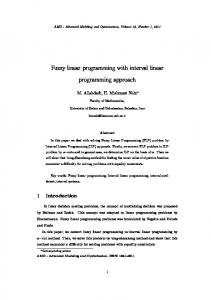
and 𝑑𝑗 ≤ 𝑑𝑗 ), respectively. The lower and upper bounds of interval number in ILP are certain as shown in Figure 1(a).
Mathematical Problems in Engineering
3
𝑑𝑈
𝑑𝐿
𝑑
𝑑
𝐿
𝑑
(a)
𝑈
̃ 𝑑
(b)
Figure 1: Interval number with certain and uncertain vertices.
The interval number of dual uncertainty linear programming is shown in Figure 1(b), and the vertices may possess a certain distribution function, such as formal distribution. The 𝑦-axis in Figure 1 does not represent any physical meaning since the figure is used to illustrate an interval number or an interval number with randomly distributed lower and upper bounds. The models (2a), (2b), (2c), and (2d) are an interval parameter linear programming with stochastic vertices, and it possesses the randomly distributed attribute of stochastic vertices and interval attribute of interval parameter; therefore, it is a dual uncertain optimization model. The traditional solution algorithm for interval-parameter linear programming (ILP) is not applicable to solve the models (2a), (2b), (2c) and (2d) due to stochastic variables existence. Considering the fuzzy features of interval number of linear programming model under dual uncertainty, a potential approach for handling such complexities in the dual uncertain linear programming framework is to introduce IFLP technique into models (2a), (2b), (2c), and (2d). This leads to an interval-parameter fuzzy linear programming with stochastic vertices (IFLPSV) model as follows:
𝑘
1 𝑈 𝐿 ∑ 𝑎𝑡𝑗 Sign (𝑎𝑈 𝑡𝑗 ) 𝑥𝑗
𝑗=1
𝑛 𝐿 + ∑ 𝑎𝑡𝑗 Sign (𝑎𝐿𝑡𝑗 ) 𝑥𝑗𝑈 𝑗=𝑘1 +1 𝑈
𝑈
𝐿
≤ 𝑏𝑡 − 𝜆 (𝑏𝑡 − 𝑏𝑡 ) , (𝑡 = 𝑠 + 1, 𝑠 + 2, . . . , 𝑚) , (3d) 𝑥𝑗𝐿 ≥ 0, 𝑥𝑗𝑈 ≥ 0,
(𝑗 = 1, 2, . . . , 𝑘1 ) ,
(3e)
(𝑗 = 𝑘1 + 1, 𝑘1 + 2, . . . , 𝑛) ,
(3f)
where 𝜆 is the fuzzy membership grade, 𝑥𝑗𝐿 (𝑗 = 1, 2, . . . , 𝑘1 ) are variables with positive coefficients in the objective function, and 𝑥𝑗𝑈 (𝑗 = 𝑘1 + 1, 𝑘1 + 2, . . . , 𝑛) are variables with negative coefficients in the objective function. 𝑓̃𝑈 and 𝑓̃𝐿 opt
max
𝜆
subject to
∑ [𝑐𝑗𝐿 + 𝑑𝑗 ] 𝑥𝑗𝐿 + ∑ [𝑐𝑗𝐿 + 𝑑𝑗 ] 𝑥𝑗𝑈
(3a)
𝑘1
𝐿
𝑗=1
𝑛
𝑗=𝑘1 +1
opt
are upper and lower bounds of objective values from models (2a), (2b), (2c), and (2d).
𝐿
(3b)
𝐿 𝑈 𝐿 ≥ 𝑓̃opt + 𝜆 (𝑓̃opt − 𝑓̃opt ), 𝑘
1 𝑈 ∑ 𝑎𝑟𝑗 Sign (𝑎𝑟𝑗𝑈) 𝑥𝑗𝐿
𝑗=1
𝑛 𝐿 + ∑ 𝑎𝑟𝑗 Sign (𝑎𝑟𝑗𝐿 ) 𝑥𝑗𝑈 𝑗=𝑘1 +1
2.2. Solving the IFLPSV. According to Huang et al. [23, 24], the above models (3a), (3b), (3c), (3d), (3e), and (3f) can be transformed into two submodels, which correspond to the upper and lower bounds of the desired objective function value. With a two-step interactive algorithm, one submodel corresponding to 𝜆𝑈 (lower bound of the membership grade) can be first formulated as max
𝜆𝑈
subject to
∑ [𝑐𝑗𝑈 + 𝑑𝑗 ] 𝑥𝑗𝑈 + ∑ [𝑐𝑗𝑈 + 𝑑𝑗 ] 𝑥𝑗𝑈
𝑘1
≤ 𝑏𝑟𝑈 − 𝜆 (𝑏𝑟𝑈 − 𝑏𝑟𝐿 ) ,
𝑗=1
(𝑟 = 1, 2, . . . , 𝑠) , (3c)
(4a) 𝑈
𝑛
𝑗=𝑘1 +1
𝐿 𝑈 𝐿 ≥ 𝑓̃opt + 𝜆𝑈 (𝑓̃opt − 𝑓̃opt ),
𝑈
(4b)
4
Mathematical Problems in Engineering 0 ≤ 𝑥𝑗𝐿 ≤ 𝑥𝑗𝑈opt ,
𝑘1
𝐿 ∑ 𝑎𝑟𝑗 Sign (𝑎𝑟𝑗𝐿 ) 𝑥𝑗𝑈
𝑥𝑗𝑈 ≥ 𝑥𝑗𝐿opt ,
𝑗=1
𝑛
𝑈 + ∑ 𝑎𝑟𝑗 Sign (𝑎𝑟𝑗𝑈) 𝑥𝑗𝐿 𝑗=𝑘1 +1
(𝑟 = 1, 2, . . . , 𝑠) , 𝑘
1 𝐿 ∑ 𝑎𝑡𝑗 Sign (𝑎𝐿𝑡𝑗 ) 𝑥𝑗𝑈
𝑗=1
𝑛 𝑈 𝐿 + ∑ 𝑎𝑡𝑗 Sign (𝑎𝑈 𝑡𝑗 ) 𝑥𝑗 𝑗=𝑘1 +1
𝑈
𝑈
(4d)
𝐿
≤ 𝑏𝑡 − 𝜆𝑈 (𝑏𝑡 − 𝑏𝑡 ) , (𝑡 = 𝑠 + 1, 𝑠 + 2, . . . , 𝑚) , 𝑥𝑗𝑈 ≥ 0, 𝑥𝑗𝐿 ≥ 0,
subject to
where 𝑥𝑗𝑈opt (𝑗 = 1, 2, . . . , 𝑘1 ), 𝑥𝑗𝐿opt (𝑗 = 𝑘1 + 1, 𝑘1 + 2, . . . , 𝑛), and 𝜆𝑈opt are solutions of models (4a), (4b), (4c), (4d), (4e), (4f), and (4g). Due to the stochastic variables existence in the models (4a), (4b), (4c), (4d), (4e), (4f), (4g), (5a), (5b), (5c), (5d), (5e), (5f), and (5g), the traditional solving algorithms of ILP (Liu et al. [18]) and DIV (Li et al. [19]) methods are impracticable. The hybrid intelligent algorithm, which incorporates ANN and GA, can be used to deal with the stochastic variables in objective function, left-hand and righthand sides of constraints. The stochastic variables of objective function and constraints need not to be initially set up, and they are automatically determined through many times iteration of the GA and ANN. Therefore, it is proposed as an intelligent algorithm. The procedure of solving the IFLPSV model by hybrid intelligent algorithm is shown in Figure 2.
(4f)
3. Illustrative Example
(4g)
The following illustrative example can be formulated to demonstrate the applicability of the proposed method:
(5a) +
max
𝑓 = [𝜉1 , 𝜉2 ] 𝑥1 − [5.5, 6.0] 𝑥2
(6a)
Subject to
[8, 10] 𝑥1 − [12, 14] 𝑥2 ≤ [𝜂1 , 𝜂2 ] ,
(6b)
𝐿 𝑑𝑗 ] 𝑥𝑗𝐿
𝑛
𝐿
+ ∑ [𝑐𝑗𝐿 + 𝑑𝑗 ] 𝑥𝑗𝐿 𝑗=𝑘1 +1
𝐿 𝑈 𝐿 ≥ 𝑓̃opt + 𝜆𝐿 (𝑓̃opt − 𝑓̃opt ),
(5b) 𝑘
1 𝑈 ∑ 𝑎𝑟𝑗 Sign (𝑎𝑟𝑗𝑈) 𝑥𝑗𝐿
𝑗=1
𝑛 𝐿 + ∑ 𝑎𝑟𝑗 Sign (𝑎𝑟𝑗𝐿 ) 𝑥𝑗𝑈 𝑗=𝑘1 +1
(5c)
≤ 𝑏𝑟𝑈 − 𝜆𝑈 (𝑏𝑟𝑈 − 𝑏𝑟𝐿 ) , (𝑟 = 1, 2, . . . , 𝑠) , 𝑘1
𝑛 𝑈 𝐿 𝐿 𝐿 𝑈 ∑ 𝑎𝑡𝑗 Sign (𝑎𝑈 𝑡𝑗 ) 𝑥𝑗 + ∑ 𝑎𝑡𝑗 Sign (𝑎𝑡𝑗 ) 𝑥𝑗
𝑗=1
𝑗=𝑘1 +1
≤
(5g)
(𝑗 = 𝑘1 + 1, 𝑘1 + 2, . . . , 𝑛) ,
𝜆𝐿 ∑ [𝑐𝑗𝐿 𝑗=1
(5f)
(4e)
With the solutions of models (4a), (4b), (4c), (4d), (4e), (4f), and (4g), another submodel corresponding to 𝜆𝐿 (lower bound of the membership grade) can be formulated as
𝑘1
(5e)
(𝑗 = 1, 2, . . . , 𝑘1 ) ,
0 ≤ 𝜆𝑈 ≤ 1.
max
(𝑗 = 𝑘1 + 1, 𝑘1 + 2, . . . , 𝑛) , 0 ≤ 𝜆𝐿 ≤ 𝜆𝑈opt ,
(4c)
≤ 𝑏𝑟𝑈 − 𝜆𝑈 (𝑏𝑟𝑈 − 𝑏𝑟𝐿 ) ,
(𝑗 = 1, 2, . . . , 𝑘1 ) ,
𝑈 𝑈 𝑏𝑡 −𝜆𝑈 (𝑏𝑡
−
𝐿 𝑏𝑡 ) ,
(𝑡 = 𝑠 + 1, 𝑠 + 2, . . . , 𝑚) , (5d)
[𝛾1 , 𝛾2 ] 𝑥1 + [3, 4] 𝑥2 ≤ [6.0, 6.5] ,
(6c)
𝑥1 , 𝑥2 ≥ 0,
(6d)
where, 𝜉1 , 𝜉2 , 𝛾1 , 𝛾2 , 𝜂1 , and 𝜂2 are the stochastic variables with normal distributions of 𝑁(26.5, 0.02), 𝑁(29.5, 0.02), 𝑁(2.4, 0.01), 𝑁(2.8, 0.01), 𝑁(3.8, 0.01), and 𝑁(4.2, 0.01), respectively. According to two-step method, the models (6a), (6b), (6c), and (6d) can be converted into two submodels. A running of the hybrid intelligent algorithm (200 iteration simulations, 500 data in ANN, and 50 generations in GA) was undertaken to solve the two sub-models. Through two-step method and hybrid artificial algorithm, the interval solutions of models (6a), (6b), (6c), and (6d) are 𝑥1 = [1.3104, 1.6401], 𝑥2 = [0.6376, 0.7748], and 𝑓 = [29.5070, 45.0840] (as shown in Table 1, no units for all results since it is only an illustrative example). Based on formulas (3a), (3b), (3c), (3d), (3e), and (3f) and Huang et al.’s [24], the models (6a), (6b), (6c), and (6d) can be converted to an IFLP problem as follows: max
𝜆
Subject to
[𝜉1 , 𝜉2 ] 𝑥1 − [5.5, 6.0] 𝑥2
(7a)
𝐿 𝑈 𝐿 ≥ 𝑓opt1 + 𝜆 [𝑓opt1 − 𝑓opt1 ],
[8, 10] 𝑥1 − [12, 14] 𝑥2 ≤ 𝜂2 − 𝜆 [𝜂2 − 𝜂1 ] ,
(7b) (7c)
Mathematical Problems in Engineering
5
Probability distribution
Discrete intervals
IFLPSV upper bound submodel
Fuzzy sets
IFLPSV model
IFLPSV lower bound submodel
Generate the training input-output dataset by random function under subject to inexact constraints
Train an ANN by the generated input-output dataset to approximate the uncertain objective function ANN
Initialization of chromosomes for GA
Select the chromosomes of GA Crossover mutation operation of GA GA
Calculate the objective value by the trained ANN
Evaluate the fitness of objective value
No
The times of cycles or the result of precision is satisfactory? Yes Generation of the decision alternatives
Figure 2: Flow chart of solving the IFLPSV model by hybrid intelligent algorithm. Table 1: Comparison of results of ILP, DIV, ILPSV, and IFLPSV method. Methods Objective value
ILP [[29.438, 32.150], [42.172, 45.784]]
DIV [[30.099, 31.455], [43.053, 44.895]]
[𝛾1 , 𝛾2 ] 𝑥1 + [3, 4] 𝑥2 ≤ 6.5 − 𝜆 [6.5 − 6.0] ,
(7d)
0 ≤ 𝜆 ≤ 1,
(7e)
𝑈 where 𝑓opt1
𝐿 and 𝑓opt1
are upper and lower bounds of objective 𝑈 value of models (6a), (6b), (6c), and (6d), 𝑓opt1 = 45.0840, and 𝐿 𝑓opt1 = 29.5070. The above models (7a), (7b), (7c), (7d), and (7e) can be solved through a two-step method where a submodel corresponding to 𝜆𝑈 is first formulated and solved. This is based on the fact that the 𝜆𝑈corresponding to 𝑓𝑈 and the system objective are to be maximized. In the second step, the other sub-model corresponding to 𝜆𝐿 can then be
ILPSV [29.5070, 45.0840]
IFLPSV [30.9548, 42.6913]
formulated supported by the solution of the first sub-model. The first sub-model can be formulated as follows: max
𝜆𝑈
Subject to
− 𝜉2 𝑥1𝑈 + 5.5𝑥2𝐿 + 15.7928𝜆𝑈
(8a)
≤ −29.2912,
(8b)
8𝑥1𝑈 − 14𝑥2𝐿 + (𝜂2 − 𝜂1 ) 𝜆𝑈 ≤ 𝜂2 ,
(8c)
𝛾1 𝑥1𝑈 + 4𝑥2𝐿 + 0.5𝜆𝑈 ≤ 6.5,
(8d)
0 ≤ 𝜆𝑈 ≤ 1.
(8e)
6
Mathematical Problems in Engineering
𝜆
max Subject to
−
(9a)
𝜉1 𝑥1𝐿
+
6.0𝑥2𝑈
+ 15.7928𝜆
≤ −29.2912, 10𝑥1𝐿 − 12𝑥2𝑈 + (𝜂2 − 𝜂1 ) 𝜆𝐿 ≤ 𝜂2 , 𝛾2 𝑥1𝐿
+
4𝑥2𝑈
𝐿
𝐿
+ 0.5𝜆 ≤ 6.5,
0.4 0.3 0.2 0.1 0
(9d)
𝑥2𝑈 ≥ 𝑥2𝐿 opt ,
(9f)
0≤𝜆 ≤
0.5
(9c)
(9e)
𝜆𝑈opt .
0.6
(9b)
𝑥1𝐿 ≤ 𝑥1𝑈opt ,
𝐿
0.7
(9g)
The solutions of models (9a), (9b), (9c), (9d), (9e), (9f), and (9g) are 𝑥1𝐿 = 1.4078 and 𝑥2𝑈 = 0.6080, and corresponding lower bound of membership grade value is 𝜆𝐿 = 0.2164 (as Figure 4). Therefore, the solutions of problem models (7a), (7b), (7c), (7d), and (7e) are 𝑥1 = [1.4078, 1.5333] and 𝑥2 = [0.6014, 0.6080], and interval objective value is 𝑓 = [30.9548, 42.6913]. In the work by Li et al. [19], dual uncertain parameters were interval values, and the DIV method was employed. The results of illustrative examples (6a), (6b), (6c), and (6d) by ILP, DIV, ILPSV, and IFLPSV method are shown in Table 1. The ILP method can tackle uncertainties expressed as interval values with known lower and upper bounds, but the distribution functions of uncertain parameters are unknown. The result of objective value from ILP is [[29.438, 32.150], [42.172, 45.784]]. The solutions might compose fuzzy information due to the parameter’s large boundary range. The DIV can tackle the uncertainties presented as interval parameter with fuzzy vertices by incorporating the vertex method within an interval parameter programming. The result of objective value from DIV is [[30.099, 31.455], [43.053, 44.895]]. Some feasible solutions might be missed by DIV method due to using the discrete vertex way, and the DIV method is unable to deal with the vertex presented as certain stochastic distribution function problem. The upper bound (42.6913) of objective value from IFLPSV is smaller than the interval [43.053, 44.895] of upper bound of DIV method. The reason is that normal distribution of upper and lower bounds of the interval parameter has more information than that of DIV model. The ILPSV method can tackle the interval-parameter linear programming with stochastic vertices. The result of objective value from IFLPSV is [30.9548, 42.6913]. The upper and lower bounds of the objective value from IFLPSV have less uncertainty than ILPSV since parameters with membership function have less
5
10
15
20 25 30 Evolution epochs
35
40
45
50
Optimal value of fitness Average value of population fitness
Figure 3: Evolution process of upper bound of membership function by genetic algorithm.
0.22 0.2 0.18 Fitness value
𝐿
0.8
Fitness value
With the hybrid intelligent algorithm, the solutions of models (8a), (8b), (8c), (8d), and (8e) are 𝑥1𝑈 = 1.5333 and 𝑥2𝐿 = 0.6014, and the corresponding upper bound of membership grade value is 𝜆𝑈 = 0.7539 (as Figure 3). Then the sub-model corresponding to 𝜆𝐿 can be formulated as follows:
0.16 0.14 0.12 0.1 0.08 0.06 0
5
10
15
20
25
30
35
40
45
50
Evolution epochs Optimal value of fitness Average value of population fitness
Figure 4: Evolution process of lower bound of membership function by genetic algorithm.
uncertainty than those with interval numbers. Furthermore, the upper and lower bounds of the objective values from IFLPSV model all lie in the interval of the upper and lower bounds from ILP model. The reason is that coefficients of IFLPSV model with fuzzy membership function and stochastic vertices have less uncertainty degree than interval parameters of ILP with interval bounds. Therefore, the uncertainty degree of the solution from the IFLPSV is also less. The developed IFLPSV model is an integrated optimization model under dual uncertainty, which considers fuzzy, interval, and stochastic attributes of parameters and coefficients of optimization model.
Mathematical Problems in Engineering
Figure 5: Location illustration of main water resources in the study area.
7 shown in formulas (10a) and (10b). The objective functions are subject to ten kinds of constraints, including water delivery capacity limit from river or lake as formula (10c), Guanting reservoir water supply capacity limit as formula (10d), Miyun reservoir water supply capacity limit as formula (10e), groundwater supply capacity limit as formula (10f), reused water supply capacity limit as formula (10g), South-toNorth Water Transfer supply capacity limit as formula (10h), the lowest requirement limit of domestic water consumption as formula (10i), the lowest requirement limit of industry water consumption as formula (10j), the lowest requirement limit of agriculture water consumption as formula (10k), the lowest requirement limit of greenbelt water irrigation as formula (10l), nonnegativity constraint is as formula (10m): 𝑚
4. Application 4.1. Overview of the Study Area. Beijing city, the capital of China, is located in the northern part of the North China Plain as shown in Figure 5. The annual precipitation is about 590 mm in Beijing, with 85% of the annual precipitation falling during the period from July to September. The main surface water source is from Guanting reservoir and Miyun reservoir in Beijing city. The amount of exploitable water resources ranges from 3.0 to 4.12 billion m3 per year. However, under changing climate and overexploitation of water resources, the total of exploitable water resources is 2.308 billion m3 in 2010 [26], including surface water resources 0.722 billion m3 and groundwater 1.586 billion m3 . The water consumption users include industry, agriculture, domestic, and environment in Beijing city. The amount of water consumption of Beijing city was 3.52 billion m3 in 2010. Water shortage problem is severe, and there has appeared four times water crisis in urbanization process of Beijing city. The per capita water resource in Beijing city is less than 300 cubic meters, which is one-thirtieth of the world average. Beijing has become one of the most water-scarce megacities in the world. Water resource has become a key factor which limits urbanization process and socioeconomic development in Beijing city. In order to meet water requirements of Northwest and North China, the South-to-North Water Diversion Projects have been developed early. The Middle Route of South-toNorth Water Diversion Project will transfer water from the Danjiangkou Reservoir on the Hanjiang river, a tributary of the Yangtze river, to Beijing city through opening channel. The Middle Route Project will be completed in 2014. The total amount of transferred water to Beijing city ranges from 1.0 to 1.4 billion m3 per year, which will be another important part of water resources for Beijing city in the future. 4.2. IFLPSV Optimization Model for Water Resources Allocation in Beijing City. Reasonable allocation of urban water resources is usually a multiobjective problem. In this study, the objective functions include net economic benefit maximization and greenbelt irrigation area maximization as
𝑛
𝑓1 = ∑ ∑ 𝑏𝑖𝑗 𝑥𝑖𝑗 (net benefit of economy) , 𝑖=1 𝑗=1 𝑚
𝑓2 = ∑ 𝑖=1
1 𝑥 (greenbelt irrigation area) , 𝑝 𝑖
(10a)
(10b)
Subject to 𝑛
∑ 𝑥𝑗 ≤ 𝑄deliv (water deliver capacity constraint
𝑗=1
from river or lake) , (10c) 𝑛
∑ 𝑥𝑗 ≤ 𝑄reser1 (Guanting reservoir water
𝑗=1
(10d)
supply capacity constraint) , 𝑛
∑ 𝑥𝑗 ≤ 𝑄reser2 (Miyun reservoir water
𝑗=1
(10e)
supply capacity constraint) , 𝑛
∑ 𝑥𝑗 ≤ 𝑄ground (groundwater supply capacity
𝑗=1
constraint) , (10f) 𝑛
∑ 𝑥𝑗 ≤ 𝑄reuse (reused water supply capacity
𝑗=1
(10g)
constraint) , 𝑛
∑ 𝑥𝑖𝑗 ≤ 𝑄trans (South-to-North Water Transfer
𝑗=1
supply capacity constraint) , (10h)
8
Mathematical Problems in Engineering 𝑚
∑ 𝑥𝑖 ≥ 𝑄domes (the lowest requirement of
(10i)
𝑖=1
domestic water consumption) , 𝑚
∑ 𝑥𝑖 ≥ 𝑄indus (the lowest requirement of 𝑖=1
𝑚
(10j)
𝑚
∑ 𝑥𝑖 ≥ 𝑄agri (the lowest requirement of 𝑖=1
agriculture water consumption) , (10k) 𝑚
𝑖=1
(10l)
greenbelt water irrigation) , 𝑥𝑖𝑗 ≥ 0 (non-negativity constraint) ,
𝐹 (𝑋) = ∑ 𝑤𝑖 𝑓𝑖 (𝑥) ,
(11)
𝑖=1
industry water consumption) ,
∑ 𝑥𝑖𝑗 ≥ 𝑄env (the lowest requirement of
The developed model is a multiobjective optimization model, including two conflict objectives. In this study, the multiobjective weighted method is adopted to solve the multi-objective model. The two objective functions are transferred to a single objective function as follows:
(10m)
where 𝑓1 , 𝑓2 are the interval objective function of the net economic benefit maximization and greenbelt irrigation area maximization, respectively, 𝑥𝑖𝑗 (𝑖 = 1, 2, 3, . . . , 𝑚; 𝑗 = 1, 2, 3, . . . , 𝑛) denotes the interval amount of water source 𝑖 supply to 𝑗 water user, 𝑚 = 6 is the total number of water source (lift or deliver water from river and lake, Guanting reservoir, Miyun reservoir, groundwater, reused water, and South-to-North Water Transfer); 𝑛 = 4 is the total number of water users (domestic, industry, agriculture and environment), 𝑏𝑖𝑗 is the benefit coefficient of the water source 𝑖 supply to 𝑗 user, which belongs an interval number, 𝑝 is the interval coefficient of greenbelt irrigation water consumption per acre, 𝑄deliv is the maximization water deliver capacity from rivers and lakes, which is an interval number, 𝑄reser1 is the water supply capacity of the Guanting reservoir, which is an interval number, 𝑄reser2 is the water supply capacity of the Miyun reservoir, which is an interval number, 𝑄ground is the groundwater supply capacity, which is an interval number, 𝑄reuse is the reused water supply capacity, which is an interval range, 𝑄trans is the available water amount from the South-to-North Water Diversion Project, which is an interval number, 𝑄domes is the lowest amount of domestic water requirement, which belongs an interval range, the reused water for domestic is small, it is ignored, 𝑄indus is the lowest amount of industry water requirement, which is an interval number, 𝑄agri is the lowest amount of agriculture water requirement, depending on weather and rainfall. The value of agriculture water requirement is an interval number with normal distribution boundaries, 𝑁(12.05 × 10⁸ , 10000) m3 and 𝑁(12.01 × 10⁸ , 10000) m3 respectively; 𝑄env is the lowest amount of greenbelt irrigation water requirement, which is an interval number. In this study, the greenbelt irrigation water requirement includes river water supplement and urban roadway watering.
where 𝑚 = 2 and 𝑤𝑖 is the weight coefficient of the 𝑖 objective function 𝑓𝑖 (𝑥), (∑𝑚 𝑖 𝑤𝑖 = 1). In this study, 𝑤1 = 𝑤2 = 0.5, and it means that economic benefit and environment protection are considered to be of the same importance. Table 2 shows the coefficients and parameters in models (10a), (10b), (10c), (10d), (10e), (10f), (10g), (10h), (10i), (10j), (10k), (10l), and (10m). The capacity of water source supply under different flow frequencies is shown in Table 3. Scenario 1 denotes the normal flow year, in which frequency of flow is 50%. The total amount of water resource is [6.184, 6.285] billion cubic meters in scenario 1. The amount of available water from local rivers and lakes is [1.38, 1.40] × 108 m3 . The available water from the Guanting and Miyun reservoirs is [7.51, 7.55] × 108 m3 and [9.15, 9.20] × 108 m3 , respectively. The amount of water from the South-to-North Middle Rout Project is [9.5, 10.0] × 108 m3 in scenario 1. Scenario 2 denotes the dry year, in which frequency of flow is 75%. The total amount of water resource is [5.751, 5.851] billion cubic meters in scenario 2, which decline 0.434 billion cubic meters comparing with scenario 1. The amount of available water from local rivers and lakes is [1.05, 1.08] × 108 m3 in scenario 2, which declines to [0.32, 0.33] × 108 m3 compared with scenario 1. The water amounts from the Guanting and Miyun reservoirs are [4.45, 4.49] × 108 m3 and [6.20, 6.24] × 108 m3 , respectively, in scenario 2, which corresponding declines to [3.06, 3.06] × 108 m3 and [3.04, 3.05] × 108 m3 compared with scenario 1. The amount of water from the South-to-North Middle Route Project is [11.5, 12.0] × 108 m3 in scenario 2, in which increase 0.2 billion cubic meters comparing with scenario 1. Scenario 3 denotes the extraordinary dry year, which frequency of flow is 90%. The total amount of water resource is [5.40, 5.50] billion cubic meters in scenario 3. The amount of available water from local rivers and lakes is [0.70, 0.72] × 108 m3 in scenario 3, in which declines to 0.68×10⁸ m3 compared with scenario 1. The amounts of water from the Guanting and Miyun reservoirs are only [1.90, 1.94] × 108 m3 and [3.60, 3.64] × 108 m3 , respectively, in scenario 3, in which declines to 5.61 × 10⁸ m3 and [5.55, 5.56] × 108 m3 compared with scenario 1. The amount of water from South-to-North Middle Route Project is [13.5, 14.0] × 108 m3 in scenario 3, which increase 0.4 billion cubic meters compared with scenario 1. The amount of exploitable groundwater and reused water keep the same for all three scenarios. 4.3. Results and Discussion. Table 4 shows the results of water allocation to water users under three scenarios. The total amount of allocated water is [6184, 6285] million m3 in
Mathematical Problems in Engineering
9 Table 2: Coefficients and parameters of model.
Water source
Domestic [4.0, 4.5] [4.0, 4.5] [4.0, 4.5] [4.0, 4.5] [0.0, 0.0] [4.0, 4.5]
Deliver water from river or lake Guanting reservoir Miyun reservoir Groundwater Reused water South-to-North Water Transfer
Benefit coefficients (RMB/m3 ) Industry Agriculture [455, 465] [0.07, 0.08] [460, 470] [0.06, 0.08] [460, 470] [0.06, 0.08] [460, 470] [0.05, 0.07] [460, 470] [0.00, 0.00] [460, 470] [0.06, 0.08]
Greenbelt irrigation ration (m3 /acre) environment [1.5, 2.0] [1.5, 2.0] [1.5, 2.0] [1.5, 2.0] [1.5, 2.0] [1.5, 2.0]
RMB: monetary symbol in China.
Table 3: Capacity of water source supply under three scenarios. Flow frequency Scenario 1 (50%) Scenario 2 (75%) Scenario 3 (90%)
Deliver water from rivers or lakes
Guanting reservoir
Miyun reservoir
Ground water
Reused water
South-to-North Water Transfer
[1.38, 1.40] [1.05, 1.08] [0.70, 0.72]
[7.51, 7.55] [4.45, 4.49] [1.90, 1.94]
[9.15, 9.20] [6.20, 6.24] [3.60, 3.64]
[26.3, 26.5] [26.3, 26.5] [26.3, 26.5]
[8.0, 8.2] [8.0, 8.2] [8.0, 8.2]
[9.5, 10.0] [11.5, 12.0] [13.5, 14.0]
Data source from [25]. (units 108 m3 ).
Table 4: Results of water resources allocation among water users under three scenarios. Scenario no. Scenario 1 (50%) Scenario 2 (75%) Scenario 3 (90%)
Domestic [1634, 1634] [1634, 1634] [1632, 1634]
Industry [2146, 2146] [1712, 1712] [1361, 1361]
Agriculture [1205, 1220] [1205, 1220] [1205, 1220]
Environment [1199, 1285] [1200, 1285] [1201, 1285]
Total water consumption [6184, 6285] [5751, 5851] [5400, 5500]
(units million m3 ).
normal flow year (50%). The total amount of allocated water is [5751, 5851] million m3 in dry year (75%), less [433, 434] million m3 than that in scenario 1. The total amount of allocated water is only [5400, 5500] million m3 in scenario 3, less [784, 785] million m3 than that in scenario 1. In Table 4 and Figure 6, the industry and domestic are main water utilization sectors in Beijing city. For example, in scenario 1, the amount of water allocation to industry is [2146, 2146] million cubic meters, which accounts for [34.1%, 34.7%] of total allocated water. The amount of allocated water to domestic is [1634, 1634] million cubic meters, which accounts for [26.0%, 26.4%] of total allocated water. In scenario 2, the amount of water allocation to industry is declined to [1712, 1712] million cubic meters, which accounts for [29.3%, 29.8%] of total allocated water. The amount of allocated water to domestic is [1634, 1634] million cubic meters, which accounts for [27.9%, 28.4%] of total allocated water. In scenario 3, the industrial water consumption is declined to [1361, 1361] million cubic meters, which only accounts for [24.7%, 25.2%] of total allocated water. The amount of allocated water to domestic is [1632, 1634] million cubic meters, which accounts for [29.7%, 30.2%] of total allocated water. Although the amount of domestic water consumption is almost not changed, its proportion is more than industrial in scenario 3. The proportion of domestic water consumption increases from [26.0%, 26.4%] in scenario 1 to [29.7%, 30.2%] in scenario 3. The results show
that domestic has higher priority than industry on water consumption under water shortage situation. The amount of water consumption of agriculture and environment reach its least requirement in Beijing city. Therefore, the amounts of agricultural and environmental water consumption are almost the same under three scenarios. In the dry year or extraordinary dry year, the water crisis might be relieved by reducing industrial water consumption. Figure 7 shows the allocation results of different water source supplies to different water users in Beijing city under three scenarios. Domestic water consumption of Beijing city is mainly from groundwater, reservoirs, and South-to-North Middle Route Project in 2020. Although the total amount of the domestic water consumption is the same under three scenarios, the amounts of water in Guanting and Miyun reservoirs (reservoir1 and reservoir 2 in Figure 2) for the domestic sector evidently decreased with rainfall reduction. Moreover, groundwater is the primary and reliable water source for the domestic sector. The allocated groundwater for domestic sector is raised from [738.2, 738.2] million m3 in scenario 1 to [764.3, 764.3] million m3 in scenario 2 and to [808.2, 808.2] million m3 in scenario 3. Meanwhile, the water amount for the domestic sector from South-toNorth Middle Route Project is raised from [325.7, 325.7] million m3 in scenario 1 to [401.8, 401.8] million m3 in scenario 2 and to [495.7, 495.7] million m3 in scenario 3. The South-to-North Middle Route Project gradually becomes
10
Mathematical Problems in Engineering
19.4%
20.9%
26.4%
20.4%
22.3%
28.4% 27.9%
22%
26%
19.5% 19.4% 21%
30.2%
23.4% 29.7%
20.9%
22.2% 22.3%
29.3%
34.1%
29.8%
34.7% Scenario 1
25.2%
Scenario 2 Agriculture Environment
Domestic Industry
24.7%
Domestic Industry
Agriculture Environment
Scenario 3 Domestic Industry
Agriculture Environment
Result of water resources allocation (million m 3 )
Figure 6: Rate of water resources allocation among water users under three scenarios. 900 800 700 600 500 400 300 200 100 0 Scenario 1 Deliver water for domestic Groundwater for domestic Deliver water for industry Groundwater for industry Deliver water for agriculture Groundwater for agriculture Deliver water for environment Groundwater for environment
Scenario 2 Reservoir 1 for domestic Reused water for domestic Reservoir 1 for industry Reused water for industry Reservoir 1 for agriculture Reused water for agriculture Reservoir 1 for environment Reused water for environment
Scenario 3 Reservoir 2 for domestic Transfer water for domestic Reservoir 2 for industry Transfer water for industry Reservoir 2 for agriculture Transfer water for agriculture Reservoir 2 for environment Transfer water for environment
Figure 7: Result of water source supply among sectors under three scenarios.
the second water source for the domestic sector when water supply capacity of the Guanting and Miyun reservoirs decreases in dry and extraordinary dry year. Industry sector mainly uses groundwater, reused water, reservoirs water, and South-to-North Middle Route Project water. The allocated water amount from these water sources for industry are all declined with total available water reducing. For example, the groundwater for industry is significantly declined, from [742.2, 742.2] million m3 in scenario 1 to [667.1, 667.1]
billion m3 in scenario 2 and to [566.8, 566.8] million m3 in scenario 3. Although the total amount of reused water supply is same, the amount of reused water for industry is declined from [496.1, 496.1] million m3 in scenario 1 to [451.1, 451.1] million m3 in scenario 2 and to [399.2, 399.2] million m3 in scenario 3. The agricultural water consumption is mainly from rivers and lakes, reservoirs, groundwater, and South-to-North Middle Route Project. Because the available water from rivers, lakes, and reservoirs is declined with
Mathematical Problems in Engineering rainfall reduction in dry year and extraordinary dry year, the exploitation amount of groundwater and South-to-North Middle Route Project water is raised to compensate water shortage of the agriculture sector. The allocated groundwater for agriculture is raised from [586.7, 599.7] million m3 in scenario 1 to [620.8, 633.8] million m3 in scenario 2 and to [679.9, 686.7] million m3 in scenario 3. The amount of South-to-North Middle Route Project water for agriculture is also raised from [187.2, 187.2] million m3 in scenario 1 to [271.3, 271.3] million m3 in scenario 2 and to [374.2, 374.2] million m3 in scenario 3. The environment mainly uses reservoirs water, groundwater, reused water, and South-toNorth Middle Route Project water. The water amount of Guanting and Miyun reservoirs for environment is declined with rainfall reduction. Contrarily, the groundwater, reused water, and transfer water for environment are all raised. For example, the reused water amount for environment is remarkably raised from [303.9, 323.9] million m3 in scenario 1 to [348.9, 368.9] million m3 in scenario 2 and to [400.8, 420.8] million m3 in scenario 3. The results show that transfer water from South-to-North Middle Route Project has significant impact on water supply structure in Beijing city. It will mitigate the water shortage issue of social and economy development in Beijing city in some extent, particularly in dry year and extraordinary dry year.
5. Conclusion An interval-parameter fuzzy linear programming with stochastic vertices (IFLPSV) has been developed for water resources allocation under dual uncertainty. The developed IFLPSV model improves upon the existing IFLP method by allowing the uncertain boundaries of interval parameter to be incorporated into the optimization processes. A hybrid intelligent algorithm based on genetic algorithm and artificial neural network was used to solve the developed model. The developed IFLPSV considers fuzzy, interval, and stochastic attributes of parameters and coefficients of objective functions and constraints. The application results indicated that it is effective for regional water resources allocation and planning under dual uncertainty. IFLPSV may provide more satisfactory solutions for an optimization problem under dual uncertainty. The developed IFLPSV model has been applied to multisource water allocation among multiple users in Beijing city in 2020, where water resources shortage is a challenging issue. The results indicate that transfering water from South-to-North Middle Route Project has an important impact on water supply structure in Beijing city, particularly in dry year and extraordinary dry year. The developed model and solution algorithm can be extended to other water resources system and environment management, where bounds of interval parameters or coefficients are dual uncertainty. In this study, only two objectives including economic and greenbelt irrigation area maximization have been considered when carrying out water allocation in Beijing city. In the future, other objectives, such as social and environmental objective, might also be involved into water resources
11 allocation in Beijing city. Moreover, interactive method for solving multi-objective optimization model is supposed to be incorporated into the methodology, so that the decision makers can make compromise among conflict objectives. There are many uncertain factors in practical management and decision making of water resources system. The interval programming is an effective method to tackle uncertainties expressed as interval values with known lower and upper bounds. However, due to high complexity of water resources system, sometimes it is hard to determine the exact values of both the lower and upper bounds. They might be with characteristics of interval, fuzzy, or random. Therefore, in this paper, the dual uncertainties are defined as interval or fuzzy numbers with lower and upper bounds with interval, fuzzy, or random characteristics. Although the bounds of interval parameters might be randomly distributed, the elements within the interval are regarded as certain numbers. In future research, physical meaning of the stochastic attribute of upper and lower bounds of interval parameters is suggested to in-depth investigation. Further discussion should be undertaken to answer whats the difference between interval number with randomly distributed bounds when the elements within the interval are simply considered as certain numbers and interval parameter as simply a random parameter with its own distribution.
Acknowledgments This research has been supported by the Open Research Fund of State Key Laboratory of Simulation and Regulation of Water Cycle in River Basin (China Institute of Water Resources and Hydropower Research). Grant no. IWHRSKL-201214, and the National Natural Science Foundation of China (no. 91125018). The authors are grateful to the editor and the anonymous reviewers for their insightful and helpful comments and suggestions.
References [1] Y. P. Li, G. H. Huang, G. Q. Wang, and Y. F. Huang, “FSWM: a hybrid fuzzy-stochastic water-management model for agricultural sustainability under uncertainty,” Agricultural Water Management, vol. 96, no. 12, pp. 1807–1818, 2009. [2] A. Abrishamchi, M. A. Marino, and A. Afshar, “Reservoir planning for irrigation district,” Journal of Water Resources Planning and Management, vol. 117, no. 1, pp. 74–85, 1991. [3] J. Kindler, “Rationalizing water requirements with aid of fuzzy allocation model,” Journal of Water Resources Planning & Management, vol. 118, no. 3, pp. 308–323, 1992. [4] J. M. Wagner, U. Shamir, and D. H. Marks, “Containing groundwater contamination: planning models using stochastic programming with recourse,” European Journal of Operational Research, vol. 77, no. 1, pp. 1–26, 1994. [5] O. Beaumont, “Solving interval linear systems with linear programming techniques,” Linear Algebra and Its Applications, vol. 281, no. 1–3, pp. 293–309, 1998. [6] P. G. Jairaj and S. Vedula, “Multi-reservoir system optimization using fuzzy mathematical programming,” Water Resources Management, vol. 14, no. 6, pp. 457–472, 2000.
12 [7] J. Q. Ma, S. Y. Chen, and L. Qiu, “A multi-objective fuzzy optimization model for cropping structure and water resources and its method,” Agriculture Science & Technology, vol. 5, no. 1, pp. 5–10, 2004. [8] I. Maqsood, G. H. Huang, and J. S. Yeomans, “An intervalparameter fuzzy two-stage stochastic program for water resources management under uncertainty,” European Journal of Operational Research, vol. 167, no. 1, pp. 208–225, 2005. [9] Y. P. Li, G. H. Huang, and S. L. Nie, “An interval-parameter multi-stage stochastic programming model for water resources management under uncertainty,” Advances in Water Resources, vol. 29, no. 5, pp. 776–789, 2006. [10] Y. P. Li, G. H. Huang, Z. F. Yang, and S. L. Nie, “IFMP: interval-fuzzy multistage programming for water resources management under uncertainty,” Resources, Conservation and Recycling, vol. 52, no. 5, pp. 800–812, 2008. [11] G. H. Huang, “A hybrid inexact-stochastic water management model,” European Journal of Operational Research, vol. 107, no. 1, pp. 137–158, 1998. [12] G. H. Huang and D. P. Loucks, “An inexact two-stage stochastic programming model for water resources management under uncertainty,” Civil Engineering and Environmental Systems, vol. 17, no. 2, pp. 95–118, 2000. [13] Q. G. Lin, G. H. Huang, B. Bass, and X. S. Qin, “IFTEM: an interval-fuzzy two-stage stochastic optimization model for regional energy systems planning under uncertainty,” Energy Policy, vol. 37, no. 3, pp. 868–878, 2009. [14] H. W. Lu, G. H. Huang, G. M. Zeng, I. Maqsood, and L. He, “An inexact two-stage fuzzy-stochastic programming model for water resources management,” Water Resources Management, vol. 22, no. 8, pp. 991–1016, 2008. [15] H. W. Lu, G. H. Huang, and L. He, “A semi-infinite analysisbased inexact two-stage stochastic fuzzy linear programming approach for water resources management,” Engineering Optimization, vol. 41, no. 1, pp. 73–85, 2009. [16] X. H. Nie, G. H. Huang, Y. P. Li, and L. Liu, “IFRP: a hybrid interval-parameter fuzzy robust programming approach for waste management planning under uncertainty,” Journal of Environmental Management, vol. 84, no. 1, pp. 1–11, 2007. [17] Z. F. Liu and G. H. Huang, “Dual-interval two-stage optimization for flood management and risk analyses,” Water Resources Management, vol. 23, no. 11, pp. 2141–2162, 2009. [18] Z. F. Liu, G. H. Huang, X. H. Nie, and L. He, “Dual-interval linear programming model and its application to solid waste management planning,” Environmental Engineering Science, vol. 26, no. 6, pp. 1033–1045, 2009. [19] Y. P. Li, G. H. Huang, P. Guo, Z. F. Yang, and S. L. Nie, “A dual-interval vertex analysis method and its application to environmental decision making under uncertainty,” European Journal of Operational Research, vol. 200, no. 2, pp. 536–550, 2010. [20] Y. Han, Y. F. Huang, and G. Q. Wang, “Interval-parameter linear optimization model with stochastic vertices for land and water resources allocation under dual uncertainty,” Environmental Engineering Science, vol. 28, no. 3, pp. 197–205, 2011. [21] B. D. Liu, Theory and Practice of Uncertain Programming, Physica, Heidelberg, Germany, 2002. [22] B. D. Liu, Theory and Practice of Uncertain Programming, Springer, Berlin, Germany, 3rd edition, 2009. [23] G. H. Huang, B. W. Baetz, and G. G. Patry, “A grey linear programming approach for municipal solid waste management
Mathematical Problems in Engineering planning under uncertainty,” Civil Engineering Systems, vol. 9, no. 4, pp. 319–335, 1992. [24] G. H. Huang, B. W. Baetz, and G. G. Patry, “A grey fuzzy linear programming approach for municipal solid waste management planning under uncertainty,” Civil Engineering Systems, vol. 10, no. 2, pp. 123–146, 1993. [25] B.-Y. Wei and J. Wang, “Analysis of water resources supply and demand in the Beijing city,” South-to-North Water Transfers and Water Science & Technology, vol. 7, no. 2, pp. 41–42, 2009 (Chinese). [26] Beijing hydrology and water resources station, Beijing water resources Bulletin, Beijing water authority, 2010.
Advances in
Operations Research Hindawi Publishing Corporation http://www.hindawi.com
Volume 2014
Advances in
Decision Sciences Hindawi Publishing Corporation http://www.hindawi.com
Volume 2014
Journal of
Applied Mathematics
Algebra
Hindawi Publishing Corporation http://www.hindawi.com
Hindawi Publishing Corporation http://www.hindawi.com
Volume 2014
Journal of
Probability and Statistics Volume 2014
The Scientific World Journal Hindawi Publishing Corporation http://www.hindawi.com
Hindawi Publishing Corporation http://www.hindawi.com
Volume 2014
International Journal of
Differential Equations Hindawi Publishing Corporation http://www.hindawi.com
Volume 2014
Volume 2014
Submit your manuscripts at http://www.hindawi.com International Journal of
Advances in
Combinatorics Hindawi Publishing Corporation http://www.hindawi.com
Mathematical Physics Hindawi Publishing Corporation http://www.hindawi.com
Volume 2014
Journal of
Complex Analysis Hindawi Publishing Corporation http://www.hindawi.com
Volume 2014
International Journal of Mathematics and Mathematical Sciences
Mathematical Problems in Engineering
Journal of
Mathematics Hindawi Publishing Corporation http://www.hindawi.com
Volume 2014
Hindawi Publishing Corporation http://www.hindawi.com
Volume 2014
Volume 2014
Hindawi Publishing Corporation http://www.hindawi.com
Volume 2014
Discrete Mathematics
Journal of
Volume 2014
Hindawi Publishing Corporation http://www.hindawi.com
Discrete Dynamics in Nature and Society
Journal of
Function Spaces Hindawi Publishing Corporation http://www.hindawi.com
Abstract and Applied Analysis
Volume 2014
Hindawi Publishing Corporation http://www.hindawi.com
Volume 2014
Hindawi Publishing Corporation http://www.hindawi.com
Volume 2014
International Journal of
Journal of
Stochastic Analysis
Optimization
Hindawi Publishing Corporation http://www.hindawi.com
Hindawi Publishing Corporation http://www.hindawi.com
Volume 2014
Volume 2014