Bayesian Ranking of Biochemical System Models - CiteSeerX
Recommend Documents
1Hugh Chipman is Associate Professor, Department of Statistics and Actuarial Science, University of Waterloo, ...... Chichester, England: John Wiley & Sons.
criterion BPR-Opt for personalized ranking ... item recommendation is to create a user-specific rank- ...... in Computer
Harry Zhang and Jiang Su. Faculty of Computer Science, University of New Brunswick ... Surprisingly, naive Bayes performs perfectly on them in ranking, even though it does ..... ing databases. Dept of ICS, University of California, Irvine (1997).
uated according to its error rate at different levels of âer- ror toleranceâ; and using medians of the absolute deviations. (MAD), rather than their mean, as the error ...
analyses of [5], and are also those given on the website for the Laub-Loomis Model, ... developed hybrid global/local optimisation algorithm to search for the ...
May 23, 2006 - these methods on the rationed credit market in Poland (Section 5). ...... Figure 2: Zloty and foreign deposits in Polish banks (in million of zlotys).
the tools of hierarchical Bayesian modeling are clearly appropriate. ... analysis is needed to manage the complexity of the tradeoffs that arise. Despite these ...
signals (i.e., music, environmental noise, speech or a mixture of these) is complex, and requires sophisticated signal processing tools. Many previous studies ...
2004 IOS Press. All rights reserved ... Considering students as an active and integral part of a learning process, models of the student become powerful tools that ...
tion of (6) is achieved (Fay and Herriot, 1979, Arora et al., 1997). .... We also consider the ''classical'' James Stein and Fay-Herriot models for the additive random ...
Hierarchical Bayesian Models for Collaborative Tagging Systems ... data complexity in these systems by finding meaningful topics that serve to group similar ...
David J.C. MacKay. In Partial Ful llment of the Requirements for the Degree of. Doctor of Philosophy. California Institute of Technology. Pasadena, California.
Department of Computer Science. National ... This paper describes a Bayesian approximation method to obtain online ranking algorithms for games ... average skill of the player (µ) and the degree of uncertainty in the player's skill (Ï). Then,.
Feb 10, 2017 - at light of SN Ia data: Akaike Information Criterion (AIC), Bayesian Information Criterion (BIC) and Bayesian Evidence (BE). These approaches ...
overview the color histogram similarity measure and the particle filter .... ËH = ( ËH1, ËH2,..., ËHn)T (consisting of the entries ËHi in ..... SHAHROKNI1/texture.html.
compared with the state-of-the-art methods such as BPR ... Figure 1: An illustration of role-based preference learning f
Nov 10, 2015 - tistical learning task, in a high dimensional setting. We propose a scoring and ranking strategy based on the PAC-Bayesian approach.
compared with the state-of-the-art methods such as BPR ... Figure 1: An illustration of role-based preference learning f
2013; Gao et al., 2013; Hu et al., 2015; Ding et al., 2015]. Furthermore, the ...... OPERA, was proposed in [Ying and Zhou, 2015], where a non-strongly convex ...
Accumulated unique developers over time as a proxy for developer engagement .... php. Cruisecontrol java. Cruisecontrol.
Jul 6, 2014 - web search engines, and the web-graphs are sparser since only a small ... best solution and may be overcome by a criteria-dependent model.
of a 10 mi/h speed limit change is provided as an example application. .... θ is a common 3-way covariance parameter among ik ..... of the studies listed here (except that in NCHRP Project 17-23) examined speeds on rural interstate highways,.
A Variable Removal Procedure. Consider the problem stated by Kano and Harada. (2000): initially, an expert provides a measure- ment/structural latent variable ...
This paper considers the Bayesian analysis of threshold regression models. ... Key words: Bayesian inference, nonlinear time series models, structural change.
Bayesian Ranking of Biochemical System Models - CiteSeerX
Dec 5, 2007 - models using realistic amounts of experimental data. Mendes et al. (2003) proposed to use artificial models for eva- luation and comparison of ...
Bioinformatics Advance Access published December 5, 2007
Bayesian Ranking of Biochemical System Models Vladislav Vyshemirsky 1,∗ and Mark A. Girolami 1 1
Department of Computing Science, University of Glasgow, Glasgow, G12 8QQ.
Associate Editor: Dr. Limsoon Wong
ABSTRACT Motivation: There often are many alternative models of a biochemical system. Distinguishing models and finding the most suitable ones is an important challenge in Systems Biology, as such model ranking, by experimental evidence, will help to judge the support of the working hypotheses forming each model. Bayes factors are employed as a measure of evidential preference for one model over another. Marginal likelihood is a key component of Bayes factors, however computing the marginal likelihood is a difficult problem, as it involves integration of nonlinear functions in multidimensional space. There are a number of methods available to compute the marginal likelihood approximately. A detailed investigation of such methods is required to find ones that perform appropriately for biochemical modelling. Results: We assess four methods for estimation of the marginal likelihoods required for computing Bayes factors. The Prior Arithmetic Mean estimator, the Posterior Harmonic Mean estimator, the Annealed Importance Sampling and the Annealing-Melting Integration methods are investigated and compared on a typical case study in Systems Biology. This allows us to understand the stability of the analysis results and make reliable judgements in uncertain context. We investigate the variance of Bayes factor estimates, and highlight the stability of the Annealed Importance Sampling and the AnnealingMelting Integration methods for the purposes of comparing nonlinear models. Availability: Models used in this study are available in SBML format as the supplementary material to this paper. Contact: [email protected]
1
INTRODUCTION
One of the important challenges of Systems Biology is inferring the structure of biochemical systems from various experimental observations (Burbeck and Jordan, 2006). Alternative models of a biochemical system can be used to describe different hypotheses about the system structure. For example, there are two alternative hypotheses about the topology of the Epidermal Growth Factor (EGF) activated MAPK pathway in PC12 cells (Roux and Blenis, 2004). The first one, supported by Brown et al. (2004) and Schoeberl et al. (2002), suggests that there is only one path involved in activating a protein named ERK when the system is stimulated with EGF. The second one, supported by Kao et al. (2001), suggests that there are two parallel paths involved in this process. These ∗ to
whom correspondence should be addressed
alternative hypotheses are described using systems of Ordinary Differential Equations (ODE). The problem is to decide which of these two alternative hypotheses is more plausible. This can be achieved by performing experiments and collecting data, and then using a statistical inferential methodology to compare the a posteriori (after observing the evidence) probabilities of the alternative models. In a diverse range of scientific disciplines, it has been shown that Bayesian Inference provides a consistent framework for knowledge updating and hypotheses testing, for example, Archaeology (Christen and Buck, 1998), Astrophysics (Brewer et al., 2007), Forensic Science (Dawid and Mortera, 1996), Bioinformatics and Computational Biology (Werhli et al., 2006; Wilkinson, 2007). In this paper we demonstrate how Bayesian hypotheses testing can be employed to rank ODE models of a biochemical system based on the evidential support they gain from experimental data and existing knowledge. The research presented in this paper is timely, as recent developments in molecular biology allow scientists to obtain more high quality experimental data vital for consistent hypotheses testing, while at the same time, the research interest of the scientific community is being shifted to study more and more complex systems (e.g. Wang et al., 2007). It is important therefore to perform reliable hypotheses testing through consistent model ranking. In this paper we assess several methods to estimate the marginal likelihood, a quantity which is required for Bayesian hypotheses testing. We consider methods which perform well on nonlinear ODE models using realistic amounts of experimental data. Mendes et al. (2003) proposed to use artificial models for evaluation and comparison of optimisation algorithms in a controlled context, where the correct result of the analysis is known. Such synthetically constructed models together with simulated data serve as a “gold standard” with which to make comparison. The technique of using artificial models for testing methodology has been widely adopted, see for example (Husmeier, 2003; Hu et al., 2007), and as such, this approach will be used in this paper.
2
APPROACH
Traditionally hypotheses about the structure of biological systems are expressed using mathematical models, typically (though not exclusively) nonlinear ordinary differential equations (Voit, 2000; de Jong, 2003). The parameters of such models are usually chosen in such a way that the predicted behaviours approach the mean of the experimental observations (see e.g. Cho et al., 2003; Schoeberl et al., 2002; Hoops et al., 2006). The Bayesian literature (e.g. Neal, 1993; Bernardo and Smith, 1994; Jaynes, 2003) argues that using probability distributions over the parameter values is a more
appropriate way of expressing the uncertainty inherent from the variability of observations. Distributions over the model parameters were successfully employed to express uncertain beliefs about parameter values by, for example, Brown et al. (2004), and more explicitly by Rogers et al. (2007) and Heron et al. (2007). Assume that alternative working hypotheses are expressed in a form of predictive parametric mathematical models. The likelihood of reproducing experimental data D, consisting of N independent identically distributed data points, with model M given a particular set of model parameters θ, and assuming Normal errors is defined as: N Y p(D|M, θ) = NDi (φ(M, θ, xi ), σ), (1) i=1
where xi is the condition in which Di was measured, and φ(M, θ, xi ) produces the value predicted with model M using parameters θ in condition xi . N· (·, ·) is the Normal probability density function, and σ 2 is the observation noise variance. Note, that a likelihood of this form is always strictly positive. This definition of the likelihood was chosen because it models the measurement noise. However, other likelihood definitions, for example Gaussian processes (Rasmussen and Williams, 2006), can be used if a more sophisticated model for the noise process is required. In the case where a discrete set of competing hypotheses is considered, they can be ranked by the ratio of their posterior probabilities. A pair of hypotheses H1 and H2 can be represented with models M1 and M2 having parameters θ1 and θ2 correspondingly. Taking a prior distribution of beliefs in preference of each model π into account, this ratio is: p(M1 |D) π (M1 ) p(H1 |D) = = × B12 p(H2 |D) p(M2 |D) π (M2 )
(2)
where B12
R p(D|M1 , θ1 ) · p(θ1 |M1 )dθ1 p (D|M1 ) R = = p (D|M2 ) p(D|M2 , θ2 ) · p(θ2 |M2 )dθ2
(3)
is called the Bayes factor for models 1 and 2. Bayes factors are used to test competing hypotheses, and update corresponding beliefs using formula (2). The Bayes factor is a summary of the evidence provided by the data in favour of one hypothesis, represented by a model, as opposed to another. Jeffreys (1961) suggested interpreting Bayes factors in half-units on the log10 scale. Pooling two of his categories together for simplification we demonstrate his scale in Table 1. Using the logarithms of the Bayes factors is often convenient, and log B12 is sometimes called the “weight of evidence in favour of H1 ”, while log likelihoods are sometimes called “surprise values”, “log evidence”, or “information content” (MacKay, 2003). Logarithmic likelihoods are measured in units of information content which depend on the base of the logarithms used1 . These categories are not a calibration of the Bayes factor, as it already provides a meaningful interpretation as probability, but rather a rough descriptive statement about standards of evidence in scientific investigation. In cases when data is uninformative due 1 ‘bit’ corresponds to log p, ‘nat’ to ln p, ‘ban’ to log 2 10 p, and ‘deciban’ to 10·log10 p. A historical overview for these names can be found in (MacKay, 2003).
2
Table 1. Interpretation of the Bayes factor as evidence support categories according to Jeffreys (1961) log10 (B) 0 to 1/2 1/2 to 1 1 to 2 >2
B 1 to 3.2 3.2 to 10 10 to 100 > 100
Evidence support Not worth more than a bare mention Substantial Strong Decisive
to, for example model overspecification, the Bayes factor will be close to 1 and thus the posterior odds do not deviate from the prior odds, thus highlighting that the experimental protocol has been uninformative. Computing Bayes factors is challenging, as the marginal likelihoods for nonlinear models have to be evaluated to obtain these. The main problem is that the marginal likelihood Z p(D|Mi ) =
p(D|Mi , θi ) · p(θi |Mi )dθi
can be evaluated analytically only in very special cases. The majority of biological models, however, are based on nonlinear ordinary differential equations. In such cases analytical integration of the marginal likelihood is impossible. Brute force numerical integration can be applied to low-dimensional problems. This approach, however, becomes computationally intractable as its complexity grows exponentially with the dimensionality of a problem The reasons of complexity leave us with the only practical option of considering methods for approximate evaluation of marginal likelihoods. Many of these approximate methods are limited by very strong conditions. For example, Laplace approximations (Bernardo and Smith, 1994) are large sample approximations around the maximum a posteriori parameter estimate. Such asymptotic approximations rely on the almost Normal density of the posterior distribution, which is often not satisfied for nonlinear problems. Two more methods which can be applied in a general case are importance sampling estimators (Newton and Raftery, 1994) and thermodynamic integration (Ogata, 1989; Gelman and Meng, 1998). Four estimators from the above classes: the Prior Arithmetic Mean estimator, the Posterior Harmonic Mean estimator, Annealed Importance Sampling and the Annealing-Melting Integration are evaluated in this paper. The first two were chosen because they are popular, straightforward to implement, and relatively inexpensive computationally. It will, however, be demonstrated in this paper that estimates produced with these estimators have large variation, and therefore cannot be used when comparing large nonlinear models. The latter two estimators are significantly more sophisticated, and have much higher computational complexity. The estimates produced with these methods are, however, significantly more stable than the ones produced with the importance sampling procedures. Importance Sampling Estimators: Importance sampling estimation consists of generating a sample from an unnormalised density π ∗ (θ). Under quite general conditions, an estimate of the integral Z p(D|M ) =
p(D|M, θ)p(θ|M )dθ
Bayesian Ranking of Biochemical System Models
is
Pm pˆ(D|M ) =
i=1
distributions
ωi · p(D|M, θ(i) ) Pm , i=1 ωi
(4)
. where ωi = p(θ(i) |M ) π ∗ (θ(i) ); the function π ∗ (θ) is known as the importance sampling function; and θ(i) is sampled from π ∗ (θ). The simplest application of this method is to use the prior as the importance sampling function π ∗ (θ) = p(θ|M ), in which case (4) produces the Prior Arithmetic Mean estimator (see McCulloch and Rossi, 1991): p(D|M ) '
m 1 X p(D|M, θ(i) ); m i=1
θ(i) ∼ p(θ|M ).
(5)
A well known problem with this estimator is that the highlikelihood region can be very small. Therefore, unless m is very large, the sample drawn from the prior will contain virtually no points from the high-likelihood region, resulting in a very poor estimate of the marginal likelihood. The problem becomes aggravated in higher dimensions, as the relative size of the high posterior probability region tends to decrease as the dimension increases. Lewis and Raftery (1997) reference a study in which to reduce the standard error to an acceptable level, it was necessary to use a sample of roughly 50 million draws from the prior distribution. An alternative application of importance sampling estimation, proposed by Newton and Raftery (1994), is to use the parameter posterior as the importance sampling function π ∗ (θ) = p(θ|D, M ). A sample from the parameter posterior can be obtained using Markov Chain Monte Carlo sampling. Such a sample should be significantly better in covering the high-likelihood region. Substituting the parameter posterior into (4) results in the Posterior Harmonic Mean estimator, we obtain: p(D|M ) '
m 1 1 X m i=1 p(D|M, θ(i) )
qβ (θ) ∝ p(D|M, θ)β p(θ|M ); 0 ≤ β ≤ 1, which form a path in the probability density space connecting the prior (when β = 0) and the posterior (when β = 1). The important feature for this estimator is that θjβ only need to be drawn approximately; thus, when using a Markov chain for producing these, the convergence of the chains to the stationary distribution is not generally required. This is a very attractive property for integrating the likelihoods of nonlinear models, as in such cases achieving convergence of the Markov chains to their stationary distributions is a very challenging problem. The following quantities are estimated from such samples: Z Zβ =
qβ (θ)dθ.
The marginal likelihood is then expanded as p(D|M ) =
Zβn Zβn−1 Zβ Z1 = ··· 1 , Z0 Zβn−1 Zβn−2 Z β0
(7)
where 0 = β0 < β1 < · · · < βn−1 < βn = 1. Each term in (7) is approximated using importance sampling based on samples from qβ (θ). The logarithm of the marginal likelihood is then estimated as: # M 1 Xˆ Ij , M j=1 # " n ” “ X (βi ) ˆ Ij = exp (βi − βi−1 ) ln p D|M, θj "
ln p(D|M ) ' ln
!−1
(8)
i=1
; (6)
θ(i) ∼ p(θ|D, M ). The main problem with this estimator is that sometimes its variance can become infinite (see the additional example provided in the supplementary material), because of the occasional occurrence of a value of θ(i) with a small likelihood and hence a large effect on the final result. For vague prior distributions, parameters in regions of high posterior mass will have high likelihood values, whilst parameters in the low posterior probability regions will tend to have low likelihood values. As the likelihood appears as a reciprocal in (6) this implies that the salient contributions to the sum come from the tails of the posterior distribution, hence the possibility of huge variances. Raftery and Newton (2007) have also demonstrated that while being asymptotically unbiased, this estimator produces biased estimates in many practical cases when finite posterior samples are used, and tends to overestimate the real value of the marginal likelihood. Annealed Importance Sampling: Neal (2001) proposed to combine importance sampling principles with the Simulated Annealing heuristic (Kirkpatrick et al., 1983). The Annealed Importance Sampling estimator can be designed to draw samples θjβ approximately from a series of unnormalised
(β )
where θj i , j = 1, . . . , M are sampled from Tβi−1 (θ|θ(βi−1 ) ), where Tβi−1 is a Markov transition kernel that has qβi−1 (θ) as its stationary distribution. Neal (2001) showed that Annealed Importance Sampling produces unbiased estimates of the marginal likelihood. Thermodynamic Integration: The logarithm of the marginal likelihood can be represented in terms of the integral Z ln p(D|M ) =
1
Eqβ (θ) [ln p(D|M, θ)] dβ.
(9)
0
This integral can be approximated by numerical integration (as in Friel and Pettitt, 2006; Lartillot and Philippe, 2006). As with Annealed Importance Sampling, this method relies on samples from unnormalised “bridging” distributions qβ (θ) which link the prior and the posterior. In the case of thermodynamic integration, a Markov chain Monte Carlo simulation is usually run for particular values of β, in which qβ is used as an unnormalised density in the Metropolis-Hastings ratio. The average of the logarithmic likelihood is then estimated on this sample. This computation is repeated for a series of values of β partitioned between 0 and 1, which implies running a separate chain for each value of β. There are a number of ways to select a schedule for β to estimate this
3
Vyshemirsky and Girolami
integral. Lartillot and Philippe (2006) use β values equally distributed between 0 and 1, whilst Friel and Pettitt (2006) use a different schedule, selecting these values as βi = aci , ai =
i , i = 0, . . . , N, N
with N = 40 and c = 4. In the example described in this paper, the latter one will be used as it produces lower variance estimates. Though, this schedule was shown to be theoretically suboptimal in general by Gelman and Meng (1998); it’s variance is superior to a uniform spacing.
3
METHODS AND RESULTS
Here we consider four alternative models of a biochemical system, with an additional example provided in the supplementary material. The models are artificially constructed to demonstrate the essence of the proposed methodology and demonstrate its main points and advantages on an example with a known result.
k1 S k2,k3
dS RS
R
k4
V, Km
(b) Model 2: A simplified version of a signal transduction cascade. It represents the same process as described by Model 1, but a mechanistic description of the activation process is omitted and replaced with more general functions.
S
dS RS
k2,k3 R
k4 Rpp
k7
RppPhA
k5,k6
PhA
(d) Model 4: A more complex version of Model 1. This model mechanistically describes how protein Rpp is deactivated by phosphotase PhA.
Fig. 1. Schematic diagrams of biochemical models used in this study.
4
is a stage in a signal transduction cascade, for example this motif is repeated several times in (Schoeberl et al., 2002). The input signal is represented by the concentration of protein S depicted in the top left of the diagram (see Fig. 1(a)). This protein activates the next stage of the cascade by binding to protein R forming complex RS, and activating R into its phosphorylated form Rpp. Protein Rpp can then be deactivated. Model 1 also defines input signal degradation by converting protein S into its degraded form dS. All the proteins used in this model will be represented as dependent variables in our ODE model. As we are interested in modelling and analysis of temporal behaviour, the independent variable is time. The dephosphorylation reaction Rpp → R is defined using the Michaelis-Menten kinetic law, while the rest of the reactions (arrows in Fig. 1(a)) are defined using the Mass Action kinetic law with parameters depicted as textual remarks beside the arrows in the model diagram (e.g. k1 , k4 ). The system of ODEs which defines this model can be found in the supplementary material. This model has six kinetic parameters: k1 . . . k4 , V, Km. plified representation of the signal transduction cascade stage. It essentially represents the same system as defined with Model 1, but uses the Michaelis-Menten kinetic law to define phosphorylation of R. The system of ODEs used in this model can be found in the supplementary material. The model has five kinetic parameters: k1 , k2 , k3 , V1 , V2 .
Model 3: The model depicted in Fig. 1(c) is a version of Model 2 with degradation of protein S removed. As protein S cannot degrade, the model would not be capable of decreasing the signal. Our goal for this model is to demonstrate through hypotheses testing, that this model gains significantly smaller evidential support from data than the rest of the models considered. The system of ODEs used in this model can be found in the supplementary material. The model has four kinetic parameters: k1 , k2 , V1 , V2 .
Model 4: The model depicted in Fig. 1(d) is a more complex version of k1
(c) Model 3: A biochemical model which is significantly different to the rest of the models considered in this paper. This model does not describe degradation of protein S.
Model 1: This model defines a common motif of signalling pathways that
Model 2: The model depicted in Fig. 1(b) was constructed as a sim-
Rpp
(a) Model 1: A model of a signal transduction cascade. Protein S represents the input signal. S can degrade to dS. At the same time S activates protein R from its inactive state, to an active state Rpp by binding and activation. Protein Rpp can then be deactivated. This model was used to generate the experimental data.
The schematic diagrams for the models are depicted in Fig. 1(a) – 1(d). The entities in circles represent proteins, while arrows correspond to biochemical reactions. Enzymatic behaviour is indicated by an arrow with a circle as head. For example, see Fig. 1(b) where S in an enzyme for activation of R. Kinetic parameters of the reactions are depicted as text beside the arrows e.g. k1 , V1 . These networks represent realistic networks, and they all have a structure which is very common in nature (Han et al., 2007). The proposed approach, however, is not limited to signal transduction applications. In the supplementary material we additionally consider the Repressilator (Elowitz and Leibler, 2000) which includes gene regulation processes, and utilises data measured in a biochemical laboratory.
Model 1. Phosphatase PhA depicted in the bottom of the diagram deactivates protein R. All the reactions are defines using the mass action kinetic law. This model was constructed to demonstrate how it would be penalised for complexity according to Occam’s razor concept (see Jaynes, 2003) in Bayesian hypotheses testing. The system of ODEs used in this model can be found in the supplementary material. This model has seven kinetic parameters: k1 . . . k7 . The initial values for all of the models can be found in SBML files provided as the supplementary material to this paper.
Data Generation: For this study we use data generated from Model 1. To generate the data we simulated the behaviour of Model 1 with the following values for kinetic parameters: k1 = 0.07
k2 = 0.6
k4 = 0.3
V = 0.017
k3 = 0.05 Km = 0.3
by solving an initial value problem, and generated the time series of variable values (protein concentrations). We decided to generate a data set for the experiments as a set of three replicates of a time series of Rpp values, measured at the following time
Bayesian Ranking of Biochemical System Models
points: t ∈ {2s, 5s, 10s, 20s, 40s, 60s, 100s}. We added observation noise with variance 0.01 to the simulated values at each of the time points. The data set D contains twenty one samples. The obtained values are depicted in Fig. 2.
[Rpp]
0.6
0.4
Table 2. Estimates of ln p(D|Mi ). PAM row corresponds to the estimates obtained with the Prior Arithmetic Mean estimator, PHM corresponds to the Posterior Harmonic Mean estimator, AIS corresponds to the Annealed Importance Sampling, and AMI corresponds to the Annealing-Melting Integration. The Posterior Harmonic Mean estimator, the Annealed Importance Sampling and the Annealing-Melting Integration methods produce the following ranking of the models: Model 1 Model 4 Model 2 Model 3. The Prior Arithmetic Mean estimates are not sufficiently separated to produce a meaningful ranking.
Fig. 2. Data set generated from Model 1. Table 3. The obtained Bayes factors.
Overall Statistical Models: The definition of the likelihood (1) has been used as described in Section 2. Only one additional noise parameter σ has been added to each of the models, as the same noise value was used when the data was generated. The same noise parameter will be substituted to the normal distributions placed at each of the time points when evaluating the likelihood (1). More sophisticated models of experimental noise can be considered if required. For example, using imunoblotting data may require a separate noise parameter for different experiments due to different affinities of the labelling antibodies; and using microarray data may require considering a log-normal distribution for experimental noise due to the saturation properties of the microarray probes. Any information about the parameter values used to generate data for our experiments with Model 1 has been discarded; and the prior for model parameters was defined. As none of the parameters can take a negative value, we defined the priors for all of the parameters of all the models to be distributed according to Gamma distribution Γ(1, 3). The mean of this prior (µ = 3) is significantly larger than any of the parameters used for data generation. Care must be taken however to ensure that the priors are not so vague that Lindley’s Paradox may become an issue. This has the effect of the Bayes factors preferring the simplest model description irrespective of the evidence to the contrary (see e.g. Denison et al., 2002, for a nice accessible discussion).
Hypotheses testing: We now compare the alternative hypotheses defined using models 1–4 by estimating corresponding marginal likelihoods and computing the Bayes factors. The Metropolis-Hasting algorithm (Hastings, 1970) was used to produce samples from distributions required for estimation of marginal likelihoods. The estimates are based on 400,000 samples drawn from each of the required distributions. We monitored the convergence of 20 parallel Markov chains to the stationary distributions for the Posterior Harmonic Mean estimator and for the Annealing-Melting Integration method for each of the βi=1...40 , using the method proposed by Gelman et al. (1995). Samples from the prior were drawn directly when required for the Prior Arithmetic Mean estimator. For the Annealed Importance Sampling we produce 4,000 proposals according to the Metropolis-Hastings algorithm β before drawing θj i . The estimates variance begins to grow if a smaller number is chosen for such “burn in”, and larger numbers do not show any benefit in the quality of the estimate. The obtained estimates (averaged from 10 repetitions for each of the models and each of the proposed estimators) for the log marginal likelihood for each of the models using each of the methods proposed above are given in Table 2. The first row of Table 2 highlights the variance of the estimates obtained using the Prior Arithmetic Mean estimator. The Posterior Harmonic Mean estimator produces larger estimates than the results obtained using the
log10 B12 7.209 “decisive”
log10 B13 20.370 “decisive”
log10 B14 4.763 “decisive”
log10 B42 2.446 “decisive”
log10 B23 13.161 “decisive”
Annealed Importance Sampling or the Annealing-Melting Integration which is consistent with (Raftery and Newton, 2007). This method in these examples, however, produces the correct relative ranking of the competing models. The variance of the estimates produced using this method may, however, become infinite, so careful monitoring of this variance is required in practice and the supplementary material provides an example demonstrating the instability of the estimator. The variances of the estimates produced by the Annealed Importance Sampling and the Annealing-Melting Integration are comparable to each other. The Annealed Importance Sampling is about 15 times faster than the Annealing-Melting Integration method on this particular example, as it requires samples to be drawn from qβ (θ) only approximately, and therefore the chains do not have to converge to their target distributions in each of these intermediate steps. Assuming equal prior distribution of beliefs between the alternative hypotheses π(M1 ) = π(M2 ) = π(M3 ) = π(M4 ), we take the mean estimates obtained with Annealing-Melting Integration (as they are the most stable) to compute the Bayes factors and use them for hypotheses testing (see Table 3). These correspond to the following relative ranking of the four competing models: Model 1 Model 4 Model 2 Model 3. The incorrect model (Model 3) gained the smallest evidential support and its marginal likelihood is dwarfed by the marginal likelihoods of other models. Model 1, which was used for data generation, has the maximal marginal likelihood, and therefore should be preferred over the rest of the models. Model 4, which was constructed to be an overly complex version of Model 1, has a smaller marginal likelihood value, and therefore is rated second. This demonstrates that Bayesian hypotheses testing accounts for the complexity of models, and implements Occam’s razor principle. According to the evidence support categories by Jeffreys (1961) defined in Table 1, the evidence suggests a “decisive” preference of the original Model 1 over the rest of the models. Interestingly, if the true model, Model 1, is not in the set being considered, we see that Model 4 Model 2, though the log B42 = 2.446 is only just decisive. This suggests both models may be considered as plausible explanation of the observed data.
5
Vyshemirsky and Girolami
4
DISCUSSION
We perform Bayesian hypothesis testing for a selection of biochemical models by computing Bayes factors. An alternative approach to this is based on the maximum a posteriori point estimates of the model parameters. Such estimates can be produced using, for example, the Simulated Annealing algorithm (Kirkpatrick et al., 1983; Hoops et al., 2006). Once such point estimates are found, the alternative models are compared by the maximised value of the corresponding posterior densities. The main problem with using maximum a posteriori estimates for model comparison is their common trend to prefer more complex models over simpler ones due to the ability of more complex models to provide a better “fit” to data. The main problem with a more general non-Bayesian hypotheses testing framework using frequentist significance tests is the obscurity of meaning for the P values (see Goodman, 1999). The smaller the P value is, the more significant the result is said to be. This value, however, is not the probability of an error. Moreover, NonBayesian tests tend to reject null hypotheses in very large samples, whereas Bayes factors do not. An example with a number of samples n = 113, 566 was discussed by Raftery (1986), where a meaningful model that explained 99.7% of the deviance was rejected by a standard χ2 test with a P value of about 10−120 but was nevertheless favoured by the Bayes factor. Akaike (1983) proposed yet another criterion for model comparison, which takes the complexity of the models into account. This criterion suggests choosing the model which minimises AIC (Akaike information criterion): AIC = −1(log maximum likelihood) + 2(number of parameters). Akaike (1983) claimed that model comparisons based on the AIC are asymptotically equivalent to those made with Bayes factors. But this is true only in the situations when predictions of the prior are compatible to those of the likelihood, and not in the more usual situation when prior information is small in comparison to the information provided by the data. Additionally, using Akaike information criterion, or similar methods, e.g. the deviance information criterion (Spiegelhalter et al., 2002), may not always provide reliable results, as these methods are justified only for the cases when parameter posteriors are unimodal and almost multivariate normal. This is a very rare case in modelling biological systems, for example, the models considered in this study are nonlinear. The non-linearity of models employed to describe alternative hypotheses is due to the fact that, in biological research, mechanistic models based on the laws of chemical kinetics are widely used. In the case when experimental data is available for only a few of the model variables (e.g. chemical species), these systems of ODEs collapse into high order differential equations, which may cause complex nonlinear likelihoods. Non-linearity of the models poses the biggest challenge for computing the marginal likelihoods required to calculate the Bayes factors, as simple methods of computing these can fail dramatically (see PAM in Table 2 and PHM in the supplementary material). In this paper we have demonstrated that such methods produce very unstable or biased results when applied to nonlinear models of biochemical systems. The reliability of such estimates will be even smaller if the parameter posterior is distributed in multiple equiprobable modes, as sampling from such distributions is very difficult.
6
On the other hand, the methods based on the principles of path sampling, for example the Annealing-Melting Integration discussed in this paper, overcome the problem of integrating difficult distributions by linking the prior, which is usually very simple to sample from, and the posterior with a path in the probability densities space. Moving along such a path helps to overcome so called energy barriers which separate local modes, and prevent Markov chains used for sampling from convergence to the true posterior distribution. These methods, however, are computationally more expensive, as Markov chains at each of the intermediate steps must converge to their stationary distributions, which may require millions of “burn-in” samples to be discarded first. We provide a comparison of the computational time required to produce one marginal likelihood estimate for Model 4 using a computer with Intel Core 2 Duo processor, PAM = 92 seconds, PHM = 145 secs, AIS = 2,187 secs, AMI = 28,703 secs. The problem of convergence becomes more and more challenging as the complexity and the size of models grow. This is a potential limitation of the applicability of the Annealing-Melting Integration estimator to only small to medium sized problems. The Annealed Importance Sampling method provides a very attractive feature that the chains do not have to converge to the stationary distributions to be useful in producing the estimates. We have demonstrated that the variance of the estimates produced with the Annealed Importance Sampling method is only marginally worse than the stability of Annealing-Melting Integration estimates, while promising faster estimation and better scalability to larger problems.
5
CONCLUSION
In this paper we considered four alternative hypotheses about the structure of a biological system defined with four realistic ODE models. All the models were artificially constructed to allow testing of the proposed methodology on an example with a known result. We simulated the experimental data from one of the suggested models; selecting the original model as the most probable one at the model comparison stage, was a crucial result to demonstrate the correctness of the approach. We demonstrated how the principle of Occam’s razor works in this framework, as the overly complex model was not preferred to the original one despite it being capable of reproducing the experimental data precisely enough. At the same time, the framework does not blindly select the simplest model. The control experiment using a structurally different model which was not capable of reproducing the general trends of system behaviour was also successful, as we demonstrated that this model was rated significantly lower as compared to the rest of the alternatives. We estimated the marginal likelihood for each of the models using four different estimators: the Prior Arithmetic Mean estimator, the Posterior Harmonic Mean estimator, the Annealed Importance Sampling and the Annealing-Melting Integration method. The estimates produced with the Prior Arithmetic Mean estimator are very unstable, while the estimates of the marginal likelihoods produced with the Posterior Harmonic Mean estimator are biased to larger values, though still capable of producing a correct ranking in this study. This demonstrates that in the cases when complex nonlinear models are employed in a study, the traditional methods of marginal likelihood estimation with importance sampling procedures may fail to provide reliable results. At the same time Annealed
Bayesian Ranking of Biochemical System Models
Importance Sampling and Annealing-Melting Integration methods provide low variance estimates. We propose to use the Annealed Importance Sampling or Annealing-Melting Integration methods in the cases when hypotheses are expressed with nonlinear ODE models. The Annealed Importance Sampling method is usually faster, as it does not require the samplers to converge when sampling from distributions bridging the prior and the posterior. At the same time, the Annealing-Melting Integration produces smaller errors of the estimates. We highlight the stability of the estimates obtained using annealing-related methods, and foresee the potential of these methods to scale to more complex applications.
ACKNOWLEDGEMENT This research is funded by Microsoft Research within the “Modelling and Predicting in Biology and Earth Sciences 2006” programme. Mark Girolami is an EPSRC Advanced Research Fellow, EP/E052029/1.
REFERENCES Akaike, H. (1983). Information measures and model selection. Bulletin of the International Statistical Institute, 50, 277–290. Bernardo, J. M. and Smith, A. F. M. (1994). Bayesian Theory. Wiley, Chichester. Brewer, B. J., Bedding, T. R., Kjeldsen, H., and Stello, D. (2007). Bayesian Inference from Observations of Solar-like Oscillations. The Astrophysical Journal, 654, 551– 557. Brown, K. S., Hill, C. C., Calero, G. A., Myers, C. R., Lee, K. H., Sethna, J. P., and Cerione, R. A. (2004). The statistical mechanics of complex signaling networks: nerve growth factor signaling. Physical Biology, 1, 184–195. Burbeck, S. and Jordan, K. E. (2006). An assessment of the role of computing in systems biology. IBM J. RES & DEV., 90(6), 529–543. Cho, K.-H., Shin, S.-Y., Kim, H.-W., Wolkenhauer, O., McFerran, B., and Kolch, W. (2003). Mathematical modeling of the influence of RKIP on the ERK signaling pathway. Lecture Notes in Computer Science, 2602, 127–141. Christen, J. A. and Buck, C. E. (1998). Sample selection in radiocarbon dating. Applied Statistics, 47(4), 543–557. Dawid, A. P. and Mortera, J. (1996). Coherent analysis of forensic identification evidence. Journal of the Royal Statistical Society, Series B, 58, 425–443. de Jong, H. (2003). Modeling and simulation of genetic regulatory systems: a literature review. Lecture Notes in Computing Science, 2602, 149–162. Denison, D., Holmes, C., Malick, B., and Smith, A. (2002). Bayesian methods for nonlinear classification and regression. Wiley. Elowitz, M. B. and Leibler, S. (2000). A synthetic oscillatory network of transcriptional regulators. Nature, 403(6767), 335–338. Friel, N. and Pettitt, A. N. (2006). Marginal likelihood estimation via power posteriors. Technical report, Department of Statistics, University of Glasgow. Gelman, A. and Meng, X.-L. (1998). Simulating normalising constants: From importance sampling to bridge sampling to path sampling. Stat. Sci., 13, 163–185. Gelman, A., Carlin, J. B., Stern, H. S., and Rubin, D. B. (1995). Bayesian Data Analysis. Chapman & Hall. Goodman, S. (1999). Toward evidence-based medical statistics. 1: The P value fallacy. Ann Intern Med, 130(12), 995–1004. Han, Z., Vondriska, T. M., Yang, L., MacLellan, W. R., Weiss, J. N., and Qu, Z. (2007). Signal transduction network motifs and biological memory. Journal of Theoretical Biology, 246(4), 755–761. Hastings, W. K. (1970). Monte Carlo sampling methods using Markov chains and thier applications. Biometrika, 57, 97–109. Heron, E. A., Finkenst¨adt, B., and Rand, D. A. (2007). Bayesian inference for dynamic transcriptional regulation; the hes1 system as a case study. Bioinformatics.
Hoops, S., Sahle, S., Gauges, R., Lee, C., Pahle, J., Simus, N., Singhal, M., Xu, L., Mendes, P., and Kummer, U. (2006). COPASI–a COmplex PAthway SImulator. Bioinformatics, 22(24), 3067–3074. Hu, J., He, X., Baggerly, K. A., Coombes, K. R., Hennessy, B. T., and Mills, G. B. (2007). Non-parametric quantification of protein lysate arrays. Bioinformatics, 23(15), 1986–1994. Husmeier, D. (2003). Sensitivity and specificity of inferring genetic regulatory interactions from microarray experiments with dynamic Bayesian networks. Bioinformatics, 19(17), 2271–2282. Jaynes, E. T. (2003). Probability Theory: The Logic Of Science. Cambridge University Press. Jeffreys, H. (1961). Theory of Probability (3rd ed.). Oxford University Press. Kao, S., Jaiswal, R. K., Kolch, W., and Landreth, G. E. (2001). Identification of the Mechanisms Regulating the Diferential Activation of the MAPK Cascade by Epidermal Growth Factor and Nerve Growth Factor in PC12 Cells. The Journal of Biological Chemistry, 276, 18169–18177. Kirkpatrick, S., Gelatt, C. D., and Vecchi, M. P. (1983). Optimization by simulated annealing. Science, 220(4598), 671–680. Lartillot, N. and Philippe, H. (2006). Computing Bayes factors using thermodynamic integration. Systematic Biology, 55(2), 195–207. Lewis, S. M. and Raftery, A. E. (1997). Estimating Bayes factors via posterior simulation with the Laplace-Metropolis estimator. J. Amer. Statist. Assoc., 92(438), 648–655. MacKay, D. J. C. (2003). Information Theory, Inference, and Learning Algorithms. Cambridge University Press. McCulloch, R. E. and Rossi, P. E. (1991). Bayes factors for nonlinear hypotheses and likelihood distributions. Technical Report 101, Statistics Research Center, University of Chicago, Graduate School of Business. Mendes, P., Sha, W., and Ye, K. (2003). Artificial gene networks for objective comparison of analysis algorithms. Bioinformatics, 19(suppl. 2), ii122–129. Neal, R. M. (1993). Probabilistic inference using Markov Chain Monte Carlo methods. Technical Report CRG-TR-93-1, Dept. of Computer Science, University of Toronto. Neal, R. M. (2001). Annealed importance sampling. Statistics and Computing, 11, 125–139. Newton, M. A. and Raftery, A. E. (1994). Approximate Bayesian inference by the weighted likelihood bootstrap. JRSS Ser. B, 3, 3–48. Ogata, Y. (1989). A Monte Carlo method for high dimensional integration. Num. Math., 55, 137–157. Raftery, A. E. (1986). Choosing models for cross-classifications. American Sociological Review, 51, 145–146. Raftery, A. E. and Newton, M. A. (2007). Estimating the integrated likelihood via posterior simulation using the harmonic mean identity. Bayesian Statistics, 8, 1–45. Rasmussen, C. E. and Williams, C. K. I. (2006). Gaussian Processes for Machine Learning. MIT Press. Rogers, S., Khanin, R., and Girolami, M. (2007). Bayesian model-based inference of transcription factor activity. BMC Bioinformatics, 8(Suppl 2:S2). Roux, P. P. and Blenis, J. (2004). ERK and p38 MAPK-Activated Protein Kinases: a Family of Protein Kinases with Diverse Biological Functions. Microbiol. Mol. Biol. Rev., 68(2), 320–344. Schoeberl, B., Eichler-Jonsson, C., Gilles, E. D., and Muller, G. (2002). Computational modelling of the dynamics of the MAP kinase cascade activated by surface and internalised EGF receptors. Nature Biotechnology, 20, 370–375. Spiegelhalter, D. J., Best, N. G., Carlin, B. P., and van der Linde, A. (2002). Bayesian measures of model complexity and fit (with discussion). JRSS Ser. B, 64(4), 583– 639. Voit, E. O. (2000). Computational Analysis of Biochemical Systems. Cambridge University Press. Wang, Y., Aguda, B. D., and Friedman, A. (2007). A continuum mathematical model of endothelial layer maintenance and senescence. Theoretical Biology and Medical Modelling, 4(30). Werhli, A. V., Grzegorcyk, M., and Husmeier, D. (2006). Comparative evaluation of reverse engineering gene regulatry networks with relevance networks, graphical Gaussian models and Bayesian networks. Bioinformatics, 22(20), 2523–2631. Wilkinson, D. J. (2007). Bayesian methods in bioinformatics and computational systems biology. Briefings in Bioinformatics, (Advance Access), 1–8.