the affinity between the images and virtual machine instances created from them. ... I. INTRODUCTION. Cloud computing is rapidly gaining momentum as a pre-.
Network Aware Virtual Machine and Image Placement in a Cloud David Breitgand
Amir Epstein
Alex Glikson
Virtualization Technologies, System Technologies & Services IBM Research - Haifa, Israel Email: {davidbr, amire, glikson}@il.ibm.com
Assaf Israel
Danny Raz
Department of Computer Science Technion, Israel Institute of Technology Email: {assafi, danny}@cs.technion.ac.il
Image Repository. The master images use RAW image format and before VM instance can be created from the template, it should be copied to a Directly Attached Storage (DAS) of the host where the new VM is to be instantiated. Since RAW image size might be in the order of gigabytes, copying RAW images from Image Repository to DAS of the hosts introduces high bandwidth overhead and long boot latencies, which offset the advantages of elastic cloud. To minimize both network bandwidth overhead and boot latency, “copy-on-write” (CoW) images are created from the master images using some CoW image format [1], [2], [3], [4]. Theoretically, a host can instantly create and boot up a minimal CoW image on DAS, pointing to the master image in the Image Repository. Thus, a new VM will write the modified data to the local DAS of the host, while using the master image for the unmodified data. Although technically possible, this configuration is rarely used in practice, because many VM instances will read the unmodified data from their master images repeatedly, introducing network overhead and read latency. Also, the Image Repository will become a bottleneck and this might limit cloud scalability. In a typical large virtualized data center from which a cloud is provided, physical machines are organized into racks, where each rack offers shared storage for storing master images that can be used by all hosts comprising the rack and also can be accessed remotely over the network by the hosts outside of the rack. The master images from the image repository are precopied into the rack storage and hosts use these master images rather than the master images stored in the Image Repository to create CoW images for VM instances. This distributed image store implementation off-loads the Image Repository service and allows to reduce traffic and latency overhead in CoW image to master image communication. In this distributed image store configuration, some VM instances are regarded local with respect to their master images, meaning that these VM instances run in the same rack where the master image resides. Other VM instances can be regarded as remote with respect to VM instances that communicate with these master images via top of the rack switch (TOR). Thanks to extreme flexibility offered by the
Abstract Optimal resource allocation is a key ingredient in the ability of cloud providers to offer agile data centers and cloud computing services at a competitive cost. In this paper we study the problem of placing images and virtual machine instances on physical containers in a way that maximizes the affinity between the images and virtual machine instances created from them. This reduces communication overhead and latency imposed by the on-going communication between the virtual machine instances and their respective images. We model this problem as a novel placement problem that extends the class constrained multiple knapsack problem (CCMK) previously studied in the literature, and present a polynomial time local search algorithm for the case where all the relevant images have the same size. We prove that this algorithm has an approximation ratio of (3 + �) and then evaluate its performance in a general setting where images and virtual machine instances are of arbitrary sizes, using production data from a private cloud. The results indicate that our algorithm can obtain significant improvements (up to 20%) compared to the greedy approach, in cases where local image storage or main memory resources are scarce. I. I NTRODUCTION Cloud computing is rapidly gaining momentum as a preferred means of providing IT at low cost. At the core of the cloud technology lies an agile data center that facilitates dynamic allocation of resources on demand to satisfy the variable hosted workloads. Although virtualization should not be equated to cloud computing, most cloud implementations use data center virtualization as the foundational technology because of the advantages it offers for dynamic reallocation of resources. It is a common practice in cloud computing to create VM instances based on “master” images, which are immutable VM templates of minimal size. Master images are stored on Network Attached Storage (NAS) in a service termed This work was partially funded by the European Commission’s 7th Framework Programme ([FP7/2003-2013]) under grant agreement no. 285248 (FIWARE Project).
ISBN 978-3-901882-53-1, 9th CNSM and Workshops ©2013 IFIP
9
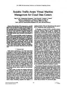
virtualization technologies, customized images with very little management effort can be created, which results in very large collections of master images. Due to the size of these master image collections it is infeasible to keep the entire collections locally to the rack where VM instances run. Therefore, the problem of minimizing network traffic overhead and latency due to communication between a CoW VM instance and its master image in a virtualized data center arises. This problem is in the focus of this study. The problem is important because CoW image to master image communication occurs in-band with the regular service traffic. Thus, scarce resources, such as network bandwidth should be managed wisely to improve goodput of the hosted applications. In the work of Tang [4], experimental evaluation demonstrated that depending on the CoW image format used, the network overhead introduced by communication between CoW image and its master image can be up to 20% and can severely impact network performance and service goodput. The need to reduce this overhead motivates works on network optimized pre-fetching of master images, e.g., [5], [4]. A typical layered network inter-connect of a data center is shown in Figure 1. Layered architecture consists of a series of connected racks. Physical servers within the same rack are connected to a top-of-rack switch. Then, the racks are connected to switches at the aggregation layer. Finally, each aggregation switch is connected with multiple switches at the core layer. In such tree topologies the available bandwidth decreases as the link level increases [6]. Thus, the average communication of a host with a storage node in the same rack is much faster than the average communication of a host with a storage node at a different rack that uses switches at higher layers. Examples of such hierarchical network topologies are tree [7], fat-tree [6] and VL2 [8]. The latter is a relatively new architecture that uses valiant load balancing to route the traffic uniformly across network paths. In this architecture the communication cost across all the racks is close to uniform.
Fig. 1.
host images) and compute capacity (i.e., resources that are required to run VM instances). We treat compute capacity as one-dimensional measure (e.g., CPU or main memory) quantifying a primary resource bottleneck. We assume that communication between VM instance and its locally placed master image is confined to the container and does not impose load on the inter-container network, while VMs communicating with their remotely placed images suffer from increased latency and introduce non-negligible overhead on the data center network. Consequently, our goal is to design efficient algorithms that make coordinated placement decisions for VM instances and their images to maximize the number of local VM instances and thus minimize the number of remote VM instances. This reduces the communication cost between virtual machine instances and their respective images. We define a novel placement problem that extends the class constrained multiple knapsack problem (CCMK) also known as data placement problem previously studied by Shachnai and Tamir [9] and Golubchik et al. [10], respectively. We introduce a new constraint, called replica constraint, that requires a feasible placement to include all images, while maximizing the number of local VM instances. Note that from the theoretical point of view this changes the problem and a new algorithmic approach is required to address it. Our model focuses on an off-line problem, where the set of demands and available machines is known. In many practical scenarios this may not be the case since requests arrive over time, however our local search algorithm can be used for initial placement of a large set of virtual machines into the the data center and for online setting as a basis for ongoing optimization that periodically improves the placement after the arrival and greedy placement of a new set of virtual machine instances by allowing migrations of virtual machines. Another important real usecase, where our proposed algorithms are beneficial arises in the context of disaster recovery. In this case a backup cluster is requested to re-establish the state of a failed cluster, based on the meta data collected about the images and VMs while the original cluster was in the operational state. It is important to be able to provide an efficient solution in this case since the resources (both in terms of computation and networking resources and in terms of time to recover) are limited. Our Main contributions are as follows. • We present a novel polynomial time local search algorithm for equal size items, and we prove that it has an approximation ratio of (3 + �). • Based on this theoretical result we develop a practical heuristic for the general setting where images and VMs are of different sizes. • We evaluate this practical algorithm using data from the private IBM research cloud. The results indicate that our proposed local search algorithm provides significant gains over a simpler algorithm that is based on a greedy packing algorithm for the problem without replica constraint.
General data center network topology
II. R ELATED W ORK The need to improve cost-efficiency by reducing capital investments into computing infrastructure and operational costs such as energy, floor space, and cooling drive the research
In this work we consider VL2-like topologies. More specifically, we assume generic containers, where each container has image capacity (i.e., the volume of the shared storage used to
ISBN 978-3-901882-53-1, 9th CNSM and Workshops ©2013 IFIP
10
the bin is at most Vj . It is also required that each item type should be assigned to at least d ≥ 1 bins. We refer to this as replica requirements. The goal is to find a feasible placement of items to the bins that maximizes the total number of packed items. This problem without the replica requirements was studied in [9], [10] and was referred as the class constrained multiple knapsack problem (CCMK) and data placement problem. The replica requirements with d > 1 might be required for fault tolerance. CCMK with replica requirements can be applied to the problem of VMs and VM images placement on physical containers in virtualized data center. Specifically, we are given a set of M VM images stored on a centralized server and N containers. Each VM image k, 1 ≤ k ≤ M is associated with a set Uk of VMs. Each container j has storage capacity Cj representing the maximum number of images that can be placed on it and load capacity Vj representing the maximum number of VMs that can be simultaneously run in it. A placement specifies for each container j, the set of VM images placed on container j and how many VM instances of each of these images are placed in container j. It is required that each image should be placed in at least one container. The goal is to find a feasible placement of all VM images and all VMs to the containers that maximizes the total number of locally placed VMs. Note that we make a natural assumption that the total compute capacity and the total image capacity of the containers is sufficient to place all the VM instances and at least one replica of each of their master images (without repetitions).
efforts on VM consolidation [11], [12], [13], [14], [15], [16] and motivate features of the products such as [17], [18], [19]. In most of the research work, VM consolidation is regarded as a classical bin packing problem where resource consumption is inferred from historical data or predicted using forecasting techniques. In addition to the primary optimization goal, which is the number of hosts, secondary goals such as migration minimization, performance optimization and other are considered. Most of this works consider physical resources such as CPU and memory. Recently, Meng et al. [20] considered consumption of network resources by VMs as an optimization goal for VM placement. They formulated the problem of assigning VMs to physical hosts to minimize the total communication costs. This goal can be achieved by placing VM pairs with large mutual traffic rate in hosts with close affinity. Another recent work used statistical multiplexing of network bandwidth among the VMs to improve VM consolidation [20], [21]. The data placement problem was considered earlier in the context of storage systems for multimedia objects such as Video-on-Demand (VOD) systems. In this problem there are n clients interested in data objects (movies) from a collection of M data objects. The system consists of N disks, where each disk j has storage capacity Cj and bandwidth (load) capacity Lj . Each client request requires a dedicated stream of one unit of bandwidth (load). This implies that each disk j can store at most Cj data objects and serve at most Lj clients of data objects stored in the disk simultaneously. The goal is to find a placement of data objects to disks and an assignment of clients to disks that maximizes the total number of served clients, subject to the capacity constraints. This problem can be modeled as the class constrained multiple knapsack problem (CCMK) also referred to as the data placement problem [9], [10]. Shachnai and Tamir [9] showed that the CCMK problem is NP-hard. They presented the moving window (MW) algorithm and showed its optimality for several interesting special cases. Golubchik et al. [10] gave a tight analysis of the moving window (MW) algorithm and provided a polynomial-time approximation scheme (PTAS) for the problem. Later, Shachnai and Tamir [22] and Kashyap and Khuller [23] studied generalizations of the problem with different item sizes. Another application of the problem is the distributed caching problem studied in [24], in which each item is a request to access data object and requires bandwidth. Requests that access the same data object instance share its storage, but requires non-shareable bandwidth.
IV. L OCAL S EARCH A LGORITHM In this section we show a polynomial time local search (3 + �)-approximation algorithm for CCMK with replica constraints. Shachnai and Tamir [9] showed that the CCMK problem is NP-hard. We first show that the CCMK problem with replica requirements is NP-hard. Theorem 4.1: The CCMK problem with replica requirements is NP-hard. Proof: We show a simple reduction from the CCMK problem without the replica constraints to the CCMK problem with replica requirements as follows. We modify the instance of CCMK to an instance of CCMK with replica constraints by adding a new bin N + 1 with capacity M and load capacity 0. Since, the load capacity of bin N + 1 is 0, in any solution to the CCMK instance with replica requirements all the items are packed in bins 1, . . . , N . Thus, it is easy to see that the number of items in the optimal solution to the CCMK instance equals the number of items in the optimal solution to the instance of CCMK with replica requirements. The problem without the replica requirements has a simple 2-approximation algorithm. For a single bin, the following greedy algorithm is optimal: Order the sets of items in nonincreasing order of sizes. Then, in step i the algorithm packs in the bin maximum number of items of set i. The algorithm terminates when reaching one of the bin capacity limits (or all items are packed in the bin). A simple greedy algorithm called Greedy for the multiple knapsack problem (MKP) is
III. M ODEL AND P ROBLEM D EFINITION We are given M item types and N bins. Each type k, 1 ≤ k ≤ M is associated with a set Uk of items. Each bin j has capacity Cj representing the maximum number of item types that can be assigned to it and load capacity Vj representing the maximum number of items that can be placed in the bin. A placement specifies for each bin j, the types of items assigned to bin j and how many items of each of these types are placed in bin j. A placement is feasible if each bin j is assigned at most Cj item types and the total number of items placed in
ISBN 978-3-901882-53-1, 9th CNSM and Workshops ©2013 IFIP
11
presented in [25]. This algorithm packs items to the bins sequentially. In step j the algorithm packs items to bin j by applying an algorithm for the single bin problem on the remaining set of items. For the CCMK problem without the replica requirements the algorithm for a single bin described above can be used by Greedy. The analysis of Greedy appears in [25] and yields the following results for our problem without the replica requirements (as previously observed in [22]). e Theorem 4.2: Greedy is a e−1 -approximation algorithm for the CCMK problem without the replica constraints and with identical bins. Theorem 4.3: Greedy is a 2-approximation algorithm for the CCMK problem without the replica constraints. We now show our local search algorithm. First we describe a 3-approximation algorithm that may have exponential running time. Then to ensure polynomial running time, we modify the algorithm to obtain a (3 + �)-approximation algorithm. Let S = (S1 , . . . , Sn ) be an assignment of items and item types to bins, where Sj is the set of items and item types assigned to bin j. The algorithm starts from an arbitrary feasible assignment of items and item types to bins such that every item type is assigned to at least d bins. The general algorithm repeatedly performs one of the following local improvements. In each step the algorithm tries to repack a single bin i from Si to Si0 or to repack a pair of bins i, j from Si , Sj to Si0 , Sj0 , respectively. Let T be the set of unassigned items. When repacking bin i or S pair of bins S i, j,Sthe algorithm considers the set of items Si T or Si Sj T , respectively for the repacking. If the repacking improves the solution then it is applied. The algorithm terminates when no further improvements are possible. The local search algorithm for the CCMK problem with replica requirements tries to replace two sets of items of different types in a bin or swap two sets of items of different types between pair of bins. The algorithm uses additional operation that combines the two operations, since there are cases where each of these operations alone may not be sufficient for improving the solution. Specifically, the algorithm, repeatedly performs one of the following local improvements. • Replace operation. Replace set of items of type k assigned to bin i with set of unassigned items of type k 0 (as illustrated by Figure 2(a)). 0 • Swap operation. Swap two sets of items of type k and k between bins i, j, respectively. Then, if there is free load capacity in bins i, j assign additional unassigned items of type k 0 , k to bins i, j, respectively (as illustrated by Figure 2(b)). Note that when a set of items is reassigned to a new bin some items may be dropped due to the load capacity limit of the bin. • Swap and Replace operation. Perform swap operation on bins i, j and then replace operation on one of the bins i or j. See Figures 2(a) and 2(b) for illustration of replace and swap operations, respectively. In this example each bin has capacity 2 and load capacity 10. There 3 items of type Pare M k and 7 items of type k 0 . Let n = k=1 |Uk | denote the total number of items. Let LS denote the value of the local
ISBN 978-3-901882-53-1, 9th CNSM and Workshops ©2013 IFIP
Fig. 2.
Local search operations.
optimum obtained by the local search algorithm and let OPT denote the value of the optimal solution. Theorem 4.4: The local search algorithm reaches a local optimal solution in O(n) steps and 3LS ≥ OP T . Proof: Let Yij be the set items of type i assigned by LS to bin j. Let Xij be the set of items of type i assigned by the optimal solutionSto bin j and are not assigned by LS to any M bin. Let Xj = i=1 Xij be the set items assigned to bin j by the optimalSsolution and are not assigned by LS to any bin M and let Yj = i=1 Yij be the set of items assigned to bin j by LS. A bin is called load saturated if it is assigned with the maximum number of items it can hold and capacity saturated if it is assigned with the maximum number of item types that it can hold. Let BL be the set of load saturated bins, let BC be the set of capacity saturated bins, which are not S load saturated and let B be the set of all bins. Let X = j and let j∈B XS S Y = j∈B Yj . Also, for a set of bins A let XA = j∈A Xj S and let YA = j∈A Yj . Let Cjf and Vjf be the free capacity and free load capacity of bin j in the local optimal solution, respectively. We now consider the set of bins BC . Recall that BC is the set of capacity saturated bins, which are not load saturated in the local optimal solution obtained by LS. We charge the set of items Y packed by LS for the set of items XBC assigned by the optimal solution to the set of bins BC and were not assigned by LS to any bin. This charging scheme is provided using the following lemma. Lemma 4.1: It holds that |XBC | ≤ |Y |. Proof: The charging scheme has two steps. In the first step we charge items assigned by LS to the set of bins BC and are of type that has strictly more than d replicas (i.e,, item type that is assigned to more than d bins) for the set of items XBC that are assigned by the optimal solution to the set of bins BC and are not assigned to any bin by LS. In the second step we charge for the subset of items in XBC that were not charged for in the first step. We now describe the details. We assume, w.l.o.g, that BC is the set of bins {1, . . . , |BC |}. For every bin j ∈ B let Yj0 ⊆ Yj be the set of items assigned by LS to bin j and are
12
Vjf . Otherwise, LS can make the following swap improvement operation. Swap the sets of items of types i1 and i between bins j and j2 . This swapSoperation replaces Yi1 j with maximal subset of items S of Yij2 Xij in bin j. We charge |Xj | items of the set Yj Yij2 for the set of items Xj (that contains Xij ). This charge is possible, since |Yj | + |Yij2 | ≥ |Yj | + |Yi1 j | + Vjf > Vj . Note that this charge replaces any charge already made for items from the set Xj . Case b: There exists a bin j2 ∈ BC and item type i2 , such that Yi2 j2 ⊆ Yj0 , |Yi2 j2 | > 0 and Yi2 j2 was not charged. Clearly, |Xij | ≤ |Yi2 j2 | (otherwise, LS can improve the solution by replacing Yi2 j2 with Xij in bin j). We charge |Xij | items of the set Yi2 j2 for the set of items Xij . Case c: There exists a bin j2 ∈ BL and an item type i2 6= i, such that Yi2 j2 ⊆ Yj0 , |Yi2 j2 | > 0 and Yi2 j2 was not charged. Let rij = min{|Xij |, |Yi1 j | + Vjf }. It must hold that |Yi2 j2 | ≥ rij . Otherwise, LS can make the following swap and replace improvement operation. First, swap the set of items Yi1 j and Yi2 j2 between bins j and j2 , respectively. Then, replace Yi2 j2 with rij items from Xij in bin j. If |Yi2 j2 | > |Xij |, then we charge |Xij | items of the set Yi2 j2 for the set of f items Xij . Otherwise, |Yj | + |Y Si2 j2 | ≥ |Yj | + Vj ≥ Vj , we charge |Xj | items of the set Yj Yi2 j2 for the set of items Xj (that contains Xij ). Note that this charge replaces any charge already made for items from the set Xj . Since all the items in the set XBC are charged for by the charging scheme and each item in the set Y is charged at most once, it follows that |XBC | ≤ |Y |. We now return to the proof of the theorem. Since all the bins in the set BL are load saturated, |XBL | ≤ |YBL |. By Lemma 4.1, |XBC | ≤ |Y |. Thus, OP T ≤ |X| + |Y | = |XBL | + |XBC | + |Y | ≤ |YBL | + 2|Y | ≤ 3|Y | = 3LS. Since each improvement step strictly increases the number of packed items, the number of improvement steps is at most n. The convergence time of the local search algorithm to a local optimum may be exponential. To ensure polynomial running time we modify the algorithm as follows. • Replace operation. Let Rkj be a set of items of type k assigned to bin j and let Rk0 j be a set of unassigned items of S type k 0 . if |Rk0 j | ≥ (1 + �)|Rkj |, then Si ← Si \ Rkj Rk0 j . • Swap operation. Let Rki and Rk0 j be sets of items of type k, k 0 assigned to bins i and j, respectively. Let Tk and Tk0 be the sets of unassigned S items of 0 type k, k 0 , S respectively. Let R Tk0Sand let 0 i ⊆ Rk 0 j k S 0 0 Rkj ⊆ Rki Tk . If S |Rk0 0 i Rkj | ≥ (1 + �)|Rki S Rk0 j |, 0 then Si ← Si \ Rki Rk0 0 i and Sj ← Sj \ Rk0 j Rkj . • Swap and Replace operation. Let Rki and Rk0 j be sets of items of type k, k 0 assigned to bins i and j, respectively. Let Tk0 and Tk00 be the sets of unassigned S items of 0 0j type k 0 , k 00 , respectively. Let R ⊆ R Tk0Sand let 0 k S 0 ki 0 Rk0 00 j ⊆ Tk00 . If |RS R | ≥ (1 + �)|R 0 00 ki S Rk0 j |, k i k j then Si ← Si \ Rki Rk0 0 i and Sj ← Sj \ Rk0 j Rk0 00 j . Note that we assume that when the algorithm performs one of the above improvement operations and assigns items of any type k to a bin, it assigns a maximal set of these items, such that the solution is feasible.
of type that has more than d replicas. Clearly, that the total capacity (or total number of types with repetitions) used by the optimal solution for the set of bins BC is at most the total capacity used by LS for the set of bins BC . Observe that if |Xij | > 0 for item type i and bin j ∈ BC then |Yij1 | = 0 for every bin j1 ∈ BC . Otherwise, LS can add items from Xij to Yij1 and thus make a local improvement. In the first step, the charging scheme iterates through the set of bins BC . In iteration j, 1 ≤ j ≤ |BC |, the charging scheme iterates through item types with set of items from Xj until all these items are considered or until all item types with set of items in Yj0 are charged once. When the charging scheme considers item type i in iteration j with |Xij | > 0, there exists an item type i1 with more than d replicas and |Yi1 j | > 0, such that Yi1 j was not charged. The charging scheme charges |Xij | items from Yi1 j for the set of |Xij | items of type i assigned by the optimal solution to bin j. Clearly, |Yi1 j | ≥ |Xij |. Otherwise, LS can make a local improvement by replacing |Yi1 j | items of type i1 with |Xij | items of type i in bin j. In the second step the charging scheme considers the subset of items from XBC that were not considered in the first step as follows. The charging scheme iterates through the set of bins BC . In iteration j, 1 ≤ j ≤ |BC |, the charging scheme iterates through item types with set of items from Xj that were not charged for in the first step. When the charging scheme considers item type i assigned by the optimal solution to bin j with |Xij | > 0, there must exists an item type i1 with set of items Yi1 j that were not charged and |Yi1 j | > 0 , since the capacity of bin j is saturated. We consider two cases. Case 1: |Yi1 j | ≥ |Xij |. Then, we charge |Xij | items from Yi1 j for the set Xij of items of type i assigned by the optimal solution to bin j. Case 2: |Yi1 j | < |Xij |. (note that item type i1 must have exactly d replicas. Otherwise, items from Yi1 j were charged in the first step of the charging scheme). In this case we will use the following observation. Observation 4.5: In case 2 the capacity of all the bins in the set B in the local optimal solution is saturated. This observation can be easily established as follows. Since, all the bins in the set BC are capacity saturated, it remains to show that the capacity of all the bins in the set BL is saturated. If there exists a bin j2 ∈ BL that is not capacity saturated then LS can make the following swap and replace improvement operation. Since bin j2 is load saturated and not capacity saturated, there exists an item type i2 with |Yi2 j2 | > 1. First, swap one item of type i2 assigned to bin j2 with the set of items of type i1 assigned to bin j. Then, replace the item of type i2 assigned to bin j with min{|Xij |, |Yi1 j | + Vjf } > Yi1 j items of type i. Thus, improving the local optimal solution. A contradiction. By observation 4.5 at least one of the following holds. • There must exist a replica of item type i2 6= i with more than d replicas that was not charged. • There exists a replica of item type i that was not charged. Now, we consider three subcases. Case a: There exists a bin j2 ∈ BL , such that |Yij2 | > 0 and Yij2 was not charged. It must hold that |Yij2 | ≥ |Yi1 j | +
ISBN 978-3-901882-53-1, 9th CNSM and Workshops ©2013 IFIP
13
with a single replica are moved between bins i and j to create a solution to the pair of bins i, j that contains only images with single replica and no items. The image movement operation may involve exhanging images between bins i and j or moving images in one direction only. Note that a single movement step might invlove multiple images on each bin. In the second step, algorithm Greedy for the multiple knapsack problem runs.
Theorem 4.6: For any � > 0, the modified local search algorithm is a polynomial time (3+�)-approximation algorithm. Proof: The proof of the approximation ratio is similar to the proof of Theorem 4.4 with the difference that each charge for a set of unassigned items is 1+� times the original charge. The polynomial running time of the algorithm follows from the fact that at each improvement step a set of items R0 replaces a set of items R, such that |R0 | ≥ (1 + �)|R|. It is easy to see that the number of steps is at most N M log1+� Vmax = O( 1� N M lnVmax ), where Vmax is the maximum load capacity of any bin. This follows from the fact that the number of sets packed in the bins is at most N M and at each improvement step one of these sets is replaced with a set larger by a factor at least 1 + �. More specifically, in replace operation a set of items is replaced with a new set larger by a factor at least 1 + �. In swap operation the size of the largest of the swapped two sets after performing the swap operation is at least 1 + � times the size of the largest of the two sets before performing the swap operation and the size of the smallest of the two sets after performing the swap operation is at least the size of the smallest of the swapped two sets before performing the swap operation.
Algorithm 1: P LACEMENT A LGORITHM Input: {(Cj , Vj )}j=1...N , {(ci , si )}i=1...n , d Output: Assignment S = (S1 , . . . , Sn ) of items to bins 1 2 3
Algorithm 2: E XTENDED G REEDY A LGORITHM : EGREEDY Input: {(Cj , Vj )}j=1...N , {(ci , si )}i=1...n , d Output: Assignment S = (S1 , . . . , Sn ) of items to bins 1 2 3
Let S be such that Sj = ∅, ∀j = 1 . . . n for k ← 1 to M do Place image k in a bin with sufficient remaining capacity
4 5
for j ← 1 to N do Apply the exact algorithm for the single bin problem on the set of remaining items (while taking into account the images packed in the previous step) return S ;
V. A P RACTICAL A LGORITHM The theoretical algorithm described in the previous section cannot be applied directly to realistic scenarios since it assumes fixed size items. Thus, we need to develop a new realistic algorithm that can handle variable size of both the VMs and the images in an efficient way. The proposed solution has two steps as described in Algorithm 1 (P LACEMENT A LGORITHM). In the first step, it computes a solution using algorithm Extended Greedy (EGREEDY, Algorithm 2). In the second step, the algorithm applies the local search procedure LS (Algorithm 3). Both algorithms are described below. Algorithm EGREEDY works as follows. In the first phase, it places each image in some container, so that by the end of this phase all images are placed. In the second phase, it runs algorithm Greedy for the multiple knapsack problem presented in Section IV. Since items have variable sizes, each knapsack optimization step in Greedy is based on the dynamic programming algorithm described in [22]. The local search procedure, LS, (see Algorithm 3) repeatedly iterates over pairs of bins in order to find local improvements in packing pairs of bins, such that the number of packed items is increased. It uses a procedure called Local(Si , Sj ) to find a repacking Si0 and Sj0 of bins i and j, respectively. If v(Si0 ) + v(Sj0 ) > v(Si ) + v(Sj ), the algorithm repacks bins i, j, where v(Si ) is the number of items in the set Si . The procedure Local finds an approximate solution to an instance of the problem with two bins (again using algorithm Greedy for the multiple knapsack problem). The procedure Local maintains the replica constraints by ensuring that images with single replica in the solution S that are packed in bins i or j are not discarded from the solution. The procedure tries improving the solution by repeatedly performing the following two steps. In the first step, images
ISBN 978-3-901882-53-1, 9th CNSM and Workshops ©2013 IFIP
S ← EGREEDY () S ← LS(S) return S ;
6
Algorithm 3: L OCAL S EARCH P ROCEDURE : LS Input: S = (S1 , . . . , Sn ), {(Cj , Vj )}j=1...N , {(ci , si )}i=1...n , d Output: Assignment S = (S1 , . . . , Sn ) of items to bins
3 4 5
while the solution was improved in the following loop do for each pair of bins i, j apply the local improvement operation do (Si0 , Sj0 ) ← Local(Si , Sj ) if v(Si0 ) + v(Sj0 ) > v(Si ) + v(Sj ) then (Si , Sj ) ← (Si0 , Sj0 )
6
return S ;
1 2
Obviously, since in a large scale setting, there are many pairs of bins to examine, the local search procedure might take too much time to execute. Moreover, at each iteration, only small improvements might be achieved. To ensure reasonable run times, we slightly modify Algorithm LS and obtain algorithm RANDOM LS as shown in Algorithm 4. At each step, it selects a random pair of bins and performs the optimization step on it. The process continues as long as there is an improvement in pair optimization. We imposed an early stopping condition that stops the optimization process if after 20 consecutive pair optimizations no improvement was achieved. To further improve the early stopping condition in a practical setting, the algorithm can be configured to stop if improvements that it achieves fell below a predefined percent of VMs in the managed environment. As indicated by the results of the next section, the randomized algorithm achieves results that are within 1% of those obtained by Algorithm 1, but with much shorter running time.
14
Algorithm 4: L OCAL S EARCH P ROCEDURE : R ANDOM LS Input: S = (S1 , . . . , Sn ), {(Cj , Vj )}j=1...N , {(ci , si )}i=1...n , d Output: Assignment S = (S1 , . . . , Sn ) of items to bins
6 7
until No improvement for 20 consecutive steps ; return S ;
90 80 Number of VM instances
4 5
repeat Select a random pair of bins i, j; Apply the local improvement operation: (Si0 , Sj0 ) ← Local(Si , Sj ) if v(Si0 ) + v(Sj0 ) > v(Si ) + v(Sj ) then (Si , Sj ) ← (Si0 , Sj0 )
1 2 3
100
70 60 50 40 30 20 10 0 1
46 91 136 181 226 271 316 361 406 451 496 541 VM Images (sorted)
VI. E XPERIMENTAL E VALUATION In this section we describe the results of experimental evaluation of the algorithm presented in the previous section. We use algorithm Extended Greedy (EGREEDY, Algorithm 2) as a baseline for comparison.
Fig. 3. Image popularity distribution: shows the number of VM instances per image. The images are sorted in order of increasing popularity.
250
A. Methodology For our evaluation, we use the data collected from a part of a private research cloud inside IBM. Specifically, we collected the data about the physical capacity (i.e., physical hosts hardware configuration), VM instances running on these hosts, images that are used to create these instances and relative image popularity. More specifically, in our setting the total number of hosts is 137. All hosts have the same amount of secondary storage (i.e., capacity), 250 GB. With respect to the amount of RAM (i.e., load capacity), the hosts are divided into four groups as described in Table I. Host Configuration Small Medium Large X-Large
Memory Capacity [GB] 30 62 126 254
Number of VMs
200
100
50
0 1
2
4
6
8
10
12
16
24
32
Memory Size (GB)
Fig. 4.
Count [%] 22 68 8 2
Total number of VM instances for each memory size (GB)
storage of the physical hosts). An intersection of each column and row shows the average improvement computed over 24 executions of the algorithm compared to the EGREEDY algorithm. Factors smaller than 0.9 are not shown in Table II, because for these factors feasible solutions do not exist in this problem instance. The standard deviation is small in all experiments. For a specific example see Table III that represents an improvement in absolute numbers for the storage factor 0.9. We used a four core 1.2 GHz per core 2007 Xeon server with 8 GB main memory to run our experiments. As one can see, the local search algorithm achieves the best results when storage is scarce. For example, when we modify the original problem instance so that the image storage takes up 90% of the host storage, the improvement of the local search algorithm ranges between 12% and 20%. We also see that the main memory is a secondary bottleneck. This result is in line with the intuition that as one has more storage capacity per host, it is easier to satisfy replica constraints and improve the affinity of VM instances and images. As main memory and secondary storage become abundant, the improvement obtained by the local search algorithm compared to the EGREEDY algorithm becomes negligible. Table III shows the results of our experiments for a fixed
TABLE I P HYSICAL H OST C ONFIGURATIONS
There are 1984 VMs in our setting. There are 10 VM sizes in use ranging from 1 to 32 GB. There are 576 master images that have at least one active VM instance. The master image popularity is shown in Figure 3. Images that do not have active VM instances are omitted from the graph. The number of VM instances per image ranges from 1 to 99 with more than half of the images having only one VM instance and a small amount of images having multiple VM instances. Figure 4 shows the number of VM instances for each memory size. As one can see most of the VMs (80%) use memory size of 2 GB and 6 GB. The image sizes range from 2 GB to 36 GB. To study the algorithm behavior we independently change capacity (i.e., the amount of local storage) and load capacity (i.e., main memory) in the original problem instance, using a uniform factor. Table II shows the results of our experiments. The columns in this table represent memory capacity factors (i.e., the uniform factors that are used to modify main memory of the physical hosts) and rows represent storage capacity factor (i.e., the uniform factors used to modify the secondary
ISBN 978-3-901882-53-1, 9th CNSM and Workshops ©2013 IFIP
150
15
Memory (GB) 0.9 1 1.1 1.2 1.3 1.4 1.5
Storage (GB) 0.9 1.0 1.2 1.089 1.19 1.074 1.18 1.07 1.16 1.059 1.14 1.042 1.12 1.026 1.12 1.015
1.1 1.093 1.072 1.065 1.057 1.037 1.022 1.017
1.2 1.052 1.049 1.043 1.031 1.019 1.0088 1.00046
1.3 1.027 1.025 1.019 1.01 1.0022 0 0
1.4 1.026 1.026 1.017 1.0075 0 0 0
for a sample execution of Algorithm 4. Both algorithms are executed for the storage and memory factors of 0.9. As one can see, in this execution both algorithms converge to essentially the same total improvement in local VM placement with Algorithm 4 being within 2% of the result of its deterministic counterpart. From the practical perspective, it is important that the optimization algorithm runs sufficiently fast for the typical cloud scales. The deterministic version of the local search passes over all bin pairs at least once. Therefore, its running time is considerably longer, 2 hours on the average as opposed to 5−6 minutes for the randomized version. Finally, we performed experiments for replica requirements of placing at least d = 2 replicas of each image that show the improvement achieved by the local search algorithm compared to the EGREEDY algorithm. These results are omitted due to space limitations.
1.5 1.021 1.025 1.016 1.0085 0 0 0
TABLE II R ANDOM L OCAL S EARCH IMPROVEMENT RATIO
storage capacity factor of 0.9 and different memory capacity factors represented by the rows of the table. The entries of the table represent the number of locally placed VMs. The second and third columns represent the average and standard deviation of the number of VMs placed by the local search algorithm, respectively. The fourth column of the table represents the number of VMs placed by EGREEDY algorithm. The last column of the table shows the average improvement in terms of number of local VMs placed by the local search algorithm compared to the EGREEDY algorithm. As one can see the standard deviation of the number of locally placed VMs placed by the local search algorithm is small. The average running time of the Random Local Search algorithm was 6 minutes with the maximum running time being 10 minutes. RAM
RANDOM Avg 1780.25 1831.25 1866.96 1900.88 1914.88 1930.33 1943.46
0.9 1 1.1 1.2 1.3 1.4 1.5
LS STD 10.74 20.25 21.60 23.40 23.9 16.0 23.27
EGREEDY
Avg Improvement
1485 1542 1589 1632 1673 1716 1741
295.25 289.25 277.96 268.88 241.88 214.33 202.46
VII. C ONCLUSIONS AND F UTURE W ORK In this work we studied the problem of maximizing affinity between VM images and VM instances created from them through joint placement of images and instances. We defined a novel optimization problem that extends the Class Constrained Multiple Knapsack problem and provide a (3 + �)approximation algorithm for it. We evaluate performance of the algorithm in a general setting where VM instances and VM images are of arbitrary sizes using production data from a private research IBM cloud. We show that the algorithm achieves significant improvements in VM instance locality when either main memory or secondary storage become a scarce resource. Future directions of this work include improvement of the approximation ratio of the presented local search algorithm, exploring the possibility of constructing an algorithm with fixed approximation ratio for the generalization of the problem where VM instances and VM images can be of arbitrary sizes. Another interesting research direction is studying the online version of the problem considering different communication costs between VMs and images, various workloads and network topologies, based on actual cloud data.
TABLE III C OMPARISON OF R ANDOM L OCAL S EARCH AND EGREEDY ALGORITHMS WITH STORAGE FACTOR OF 0.9
1900
R EFERENCES
1800
1700
[1] M. McLoughlin, “The QCOW2 Image Format,” http://people.gnome.org/ ∼markmc/qcow-image-format.html. [2] “VMware Virtual Disk Format 1.1,” http://www.vmware.com/ technical-resources/interfaces/vmdk.html. [3] “Microsoft VHD Image Format,” http://technet.microsoft.com/en-us/ virtualserver/bb676673.aspx. [4] C. Tang, “FVD: A high-performance virtual machine image format for cloud,” in USENIX ATC. Portland, OR, USA: USENIX, Jun 2011. [5] C. Peng, M. Kim, Z. Zhang, and H. Lei, “VDN: Virtual machine image distribution network for cloud data centers,” in INFOCOM, 2012 Proceedings IEEE, march 2012, pp. 181 –189. [6] M. Al-Fares, A. Loukissas, and A. Vahdat, “A scalable, commodity data center network architecture,” in SIGCOMM, 2008, pp. 63–74. [7] Juniper, “Cloud-ready data center reference architecture,” http://www. juniper.net/us/en/local/pdf/reference-architectures/8030001-en.pdf. [8] A. G. Greenberg, J. R. Hamilton, N. Jain, S. Kandula, C. Kim, P. Lahiri, D. A. Maltz, P. Patel, and S. Sengupta, “Vl2: a scalable and flexible data center network,” Commun. ACM, vol. 54, no. 3, pp. 95–104, 2011. [9] H. Shachnai and T. Tamir, “On two class-constrained versions of the multiple knapsack problem,” Algorithmica, vol. 29, no. 3, pp. 442–467, 2001.
Number of VMs
1600
1500
LS
1400
Random LS
1300
1200
1100
1000 1
21
41
61
81
101
121
141
Improvment steps
Fig. 5. Total number of placed VMs in each LS improvement step for storage and memory factors of 0.9
Figure 5 shows improvements in number of locally placed VMs per improvement step for Algorithm 3 and Algorithm 4
ISBN 978-3-901882-53-1, 9th CNSM and Workshops ©2013 IFIP
16
[10] L. Golubchik, S. Khanna, S. Khuller, R. Thurimella, and A. Zhu, “Approximation algorithms for data placement on parallel disks,” in SODA, 2000, pp. 223–232. [11] A. Verma, P. Ahuja, and A. Neogi, “pmapper: power and migration cost aware application placement in virtualized systems,” in Middleware ’08: Proceedings of the 9th ACM/IFIP/USENIX International Conference on Middleware. New York, NY, USA: Springer-Verlag New York, Inc., 2008, pp. 243–264. [12] S. Mehta and A. Neogi, “Recon: A tool to recommend dynamic server consolidation in multi-cluster data centers,” in IEEE Network Operations and Management Symposium (NOMS 2008), Salvador, Bahia, Brasil, Apr 2008, pp. 363–370. [13] J. E. Hanson, I. Whalley, M. Steinder, and J. O. Kephart, “Multi-aspect hardware management in enterprise server consolidation,” in NOMS, 2010, pp. 543–550. [14] S. Srikantaiah, A. Kansal, and F. Zhao, “Energy aware consolidation for Cloud computing,” in HotPower 08 Workshop on Power Aware computing and Systems, San Diego, CA, USA, 2008. [15] Y. Ajiro and A. Tanaka, “Improving packing algorithms for server consolidation,” in International Conference for the Computer Measurement Group (CMG), 2007. [16] S. Chen, K. R. Joshi, M. A. Hiltunen, R. D. Schlichting, and W. H. Sanders, “CPU gradients: Performance-aware energy conservation in multitier systems,” in Green Computing Conference, 2010, pp. 15–29. [17] VMware Inc., “Resource Management with VMware DRS, Whitepaper,” 2006. [18] IBM, “Server Planning Tool,” http://www-304.ibm.com/jct01004c/ systems/support/tools/systemplanningtool/. [19] ——, “WebSphere CloudBurst,” http://www01.ibm.com/software/webservers/cloudburst/. [20] M. Wang, X. Meng, and L. Zhang, “Consolidating virtual machines with dynamic bandwidth demand in data centers,” in INFOCOM, 2011. [21] D. Breitgand and A. Epstein, “Improving consolidation of virtual machines with risk-aware bandwidth oversubscription in compute clouds,” in INFOCOM, 2012. [22] H. Shachnai and T. Tamir, “Approximation schemes for generalized 2-dimensional vector packing with application to data placement,” in RANDOM-APPROX, 2003, pp. 165–177. [23] S. R. Kashyap and S. Khuller, “Algorithms for non-uniform size data placement on parallel disks,” J. Algorithms, vol. 60, no. 2, pp. 144–167, 2006. [24] L. Fleischer, M. X. Goemans, V. S. Mirrokni, and M. Sviridenko, “Tight approximation algorithms for maximum general assignment problems,” in SODA, 2006, pp. 611–620. [25] C. Chekuri and S. Khanna, “A polynomial time approximation scheme for the multiple knapsack problem,” SIAM J. Comput., vol. 35, no. 3, pp. 713–728, 2005.
ISBN 978-3-901882-53-1, 9th CNSM and Workshops ©2013 IFIP
17