Virtual Machine Placement Using Biogeography

Virtual Machine Placement Using Biogeography-Based Optimization Qinghua Zhenga,b , Rui Lia,b , Xiuqi Lic , Nazaraf Shahd , Jianke Zhanga,e , Feng Tiana,f , Kuo-Ming Zhaod , Jia Lia,b a MOE

Key Lab for Intelligent Networks and Network Security, Xi’an Jiaotong University, Xi’an, China; of Computer Science and Technology, Xi’an Jiaotong University, Xi’an, China; c Department of Computer Science and Mathematics, University of North Carolina at Pembroke, Pembroke, NC 28372, USA; d Faculty of Engineering and Computing, Coventry University, UK; e School of Science, Xi’an University of Posts and Telecommunications, Xi’an 710121, China; f Systems Engineering Institute, Xi’an Jiaotong University, Xi’an, China; b Department

Abstract Virtual machine placement (VMP) is an important issue in selecting the most suitable set of physical hosts for a set of virtual machines in cloud computing environment. VMP problem consists of two sub problems: incremental placement (VMiP) problem and consolidated placement (VMcP) problem. The challenge in VMcP problem is how to find optimal solution effectively and efficiently as well as it is a kind of NP-hard problem. In this paper, we present a novel solution to the VMcP problem called VMPMBBO. The scheme of VMPMBBO treats the VMcP problem as a complex system, and utilizes the biogeography-based optimization (BBO) technique to optimize the virtual machine placement that minimizes both the resource waste and the power consumption at the same time. Extensive experiments are conducted using synthetic data from related literature and data from two real datasets. First of all, the necessity of VMcP has been proved by experimental results obtained by applying VMPMBBO. Then, the proposed method is compared with two existing multi-objective VMcP optimization algorithms and it is shown that VMPMBBO has better convergence characteristics and is more computationally efficient. VMPMBBO is also robust. And then, the issue of parameter setting of the proposed method has been discussed. Finally, adaptability and extensibility of VMPMBBO have also been proved. To the best of our knowledge, this work is the first approach that applies biogeography-based optimization (BBO) to virtual machine placement (VMP). Keywords: Virtual machine placement, Multi-objective optimization, Resource utilization, Biogeography-based optimization, Cloud computing

1. Introduction Cloud computing has been a popular computing paradigm in IT industry since 2008. It delivers computing infrastructures, computing platforms, and software as hosted services on demand over the Internet. Cloud users can access computing resources without having to own, manage, and maintain them. There are three common cloud computing models known as Infrastructure-as-a-Service (IaaS), Platform-as-a-Service (PaaS), and Software-as-a-Service (SaaS) [1, 2, 3]. In the most basic model IaaS like Amazon Web Services, cloud users are provided with physical or more often virtual servers and additional resources like raw block storage, which are allocated from massive computing resource pools in large-scale data centers. The focus of this paper is on IaaS model. From the perspective of a cloud provider, to reduce the operating cost, the use of computing resources in cloud needs to be maximized. In addition, the power consumption needs to be minimized as it became a significant contributor to the operating cost [4]. The total electricity used by data centers in the US increased about 56% from 2005 to 2010 [5]. The core technology in cloud computing is virtualization [6], which separates resources and services from the underlying physical delivery environment. The resources of a single physical machine (PM) are sliced into multiple isolated execution environments for multiple virtual machines (VMs). Virtual Machine Placement (VMP) is an important topic in cloud environment virtualization, in particular in IaaS model. VMP maps a set of virtual machines to a set of physical machines. For the cloud providers, a good VMP solution should maximize resource utilization and minimize power consumption. Preprint submitted to Future Generation Computer Systems

January 19, 2015

... VMiP

continus VM requests (deployment requests & removal requests)

deploy/remove VM

PM

PM

PM

...

PM

PM

PM

...

PM

PM

PM

...

PM

PM

PM

...

VMcP consolidate VMs

Fig. 1: An example of VMiP and VMcP

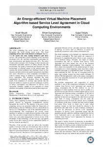
The problem of VMP consists of two sub problems: incremental placement (VMiP) problem and consolidated placement (VMcP) problem [7], as shown in Fig. 1. VMiP is deals with continuous arrival of VM deployment requests in runtime. Quick response is a crucial metric for ensuring a high service quality of the VMiP. The problem of VMiP has received much attention [8, 9, 10, 7]] as VMs are being continuously removed over time, which may bring the infrastructure to a poor state over a long time period. Therefore, it is necessary to consolidate VMs into servers periodically [7]. One of the benefits of virtualization is the ability of readjusting existing VMs into the more suitable servers. This process, known as VMcP, is used by data centers to increase resource utilization and reduce electric power consumption costs [11]. VMcP is particularly important when user workloads are unpredictable and VMP need to be revisited periodically [11]. Whenever VM instances change, VMs can be relocated and migrated to different physical servers if necessary [11]. VMcP can be invoked periodically, or be triggered based on some preset conditions. The problem of VMcP is NP-hard [12, 13, 14, 15, 16, 17]. The challenge in VMcP problem is how to find optimal solution effectively and efficiently as well as it is a kind of NP-hard problem. The existing research in VMcP can be classified into five categories based on the techniques being used: heuristic bin packing [18, 19, 20, 21, 22, 23, 24, 25, 12, 26], biology-based optimization [27, 28, 29, 30, 31, 32], linear programming [33, 34], constraint programming [35], and simulated annealing optimization [36]. Another kind of classification is single-objective or multi-objective based on number of objectives to be optimized during the placement. Recent research [5, 31, 37] focus on multi-objective solutions. Both [5] and [31] optimize resource utilization and power consumption. The thermal dissipation cost is also considered in some research efforts [31]. The work in [37] optimizes CPU utilization, network throughput, and disk I/O rate. Existing biology-based optimization algorithms for VMcP include genetic algorithms [29, 5], particle swarm optimization [28] and ant colony optimization [27, 31]. In this paper, we propose a novel multi-objective VMcP solution named VMPMBBO. It employs a state-of-theart evolutionary algorithm, biogeography-based optimization (BBO) [38, 39] to find the optimal VM placements that simultaneously minimizes both the resource waste and the power consumption. Compared with two existing multi-objective evolutionary algorithms [5, 31], VMPMBBO has better convergence characteristics and is more computationally efficient. Extensive simulation results confirm the effectiveness, efficiency and robustness of the proposed approach. Adaptability and extensibility of VMPMBBO have also been proved by experimental results. To the best of our knowledge, this work is the first approach that applies biogeography-based optimization (BBO) and complex system optimization to virtual machine placement (VMP). The remainder of this paper is organized as follows. In Section 2, the existing VMP solutions are reviewed. VM placement problem is formulated in Section 3. Section 4 presents background knowledge of the proposed VMPMBBO approach. The simulation results are presented in Section 4. Section 5 evaluates the effectiveness of the proposed approach. Section 6 proves the adaptability and extensibility of VMPMBBO and finally Section 7 concludes the paper.

2

2. Related Work VMcP is one the well research area in cloud computing [4, 18, 19, 20, 27, 28, 29, 30, 31]. These research efforts can be classified into five categories based on their underlying techniques: heuristic bin packing [18, 19, 20, 33, 21, 22, 23, 24, 25, 12, 26], biology-based optimization [27, 28, 29, 30, 31, 32], linear programming [33, 34], constraint programming [35], and simulated annealing optimization [36]. Heuristic bin packing Many studies model the VM placement as vector bin packing, a well- known NP-hard optimization problem [19]. Simple heuristics like greedy algorithms are utilized to approximate the optimal solution of this NP-hard problem. These include worst fit and best fit in [18], first fit decreasing (FFD) and best fit decreasing (BFD) [33, 22]. An extended first fit decreasing (FFD) heuristics in the pMapper system [20, 39], first fit and best fit modified using node utility and power consumption [21], worst fit based on the profiling data [23], first fit modified using application migration [24], best fit used for VM migration in [12], and a modified best fit decreasing heuristics in [26]. Biology-based Optimization. In [27], an ant colony optimization method (ACO) is used to pack the VMs to the least number of physical machines necessary for the current workload. The SAPSO approach [28, 32] is a self-adaptive particle swarm optimization (PSO) algorithm. SAPSO has been applied to automatically adjusts VM placement in response to changing resource pools in a dynamic cloud environment. The GABA approach [29] is a genetic algorithm (GA) based algorithm that dynamically reconfigures the VM mappings according to estimated future workload in a dynamic cloud environment. Linear programming. In [33], the server consolidation problem is considered as bin packing, for which FFD and BFD are suggested. In addition, the server consolidation problem is formulated as linear programming that is extended with a number of constraint types elicited from practical applications. An LP-relaxation-based heuristic is designed to minimize the cost of linear programming. The study in [34] formulates the QoS-aware VMP problem as integer linear programing (ILP) and proposes a polynomial-time heuristic algorithm based on bipartite graph to reduce the complexity of ILP and efficiently solve the problem. Constraint programming. A resource management framework is presented in [35]. It consists of two major components, a dynamic utility-based VM provisioning manager and a dynamic VM placement manager. Both managing tasks are modeled as constraint satisfaction problems. Entropy is a resource manager [40] used for homogeneous clusters, which employs constraint programing to perform dynamic consolidation and considers both VM placement and VM migration. Simulated annealing optimization. The authors in [36] propose a dynamic runtime virtual machine mapping framework called GreenMap that contains multiple modules. The placement module utilizes a simulated annealing optimization based algorithm to dynamically map the VMs onto a small set of PMs that minimizes power consumption without significantly degrading the system performance. Many VMcP schemes optimize a single objective such as resource utilization, power consumption or load balancing, etc. However, real-world VMcP solutions often need to consider multiple objectives. Take VMcP as an example, its optimization model of has been widely studied and a number of characteristics have been taken into consideration, according to the specific application scenarios, such as, VM dependency [41], inter-VM data movement [41, 42, 43] and load balance [44, 45, 46, 47]. The characteristics considered in these research efforts have been formalized as objective functions or constraints. Meanwhile,recent research efforts tend to adopt evolutionary algorithm to address this kind multi-objective optimization problem. MGGA in [5] employs a grouping genetic algorithm with fuzzy multiobjective evaluation to minimize the resource waste, power consumption, and the thermal dissipation costs. VMPACS in [31] is a multi-objective ant colony system algorithm (ACO) that minimizes both the total resource waste and the power consumption. The work in [37] optimizes CPU utilization, network throughput, and disk I/O rate using a hybrid genetic algorithm for VMcP. This paper firstly incorporates five factors into the optimization model, which is more complex than the ones in above research. 3. Problem formulation The first part of this section describes a universal resource waste model, which supported multiple resource dimensions. And then, a power consumption model has been built based on literatures and experiments. Finally we formalize VMcP optimization problem. 3

3.1. Resource Waste Model Different VMcP solutions may leave different amount of residual resources for each resource type on each PM. To accommodate future requests, an effective VMcP solution should keep the residual resources balanced in each dimension. Fig. 2 illustrated the balanced problem of residual resources. The cube represents the total CPU, memory and bandwidth capacity of a server. The two small cubes labeled VM1 and VM2 represent the amount of CPU, memory and bandwidth allocated to the two VMs. The left small cube labeled Residual Capacity denotes the remaining amount of CPU, memory and bandwidth after placing two VMs. Clearly, there is a lot of memory and bandwidth left but little CPU remaining. This CPU scarcity may block the placement of a new VM on this server.

Bandwidth

Residual Capacity

VM 2

VM 1

Me

mo

ry

CPU Fig. 2: An example of resources allocated to two VMs placed into a single PM

Based on the above observation, we propose resourceWaste( j) function to quantify the cost of resource waste in the multiple loads on a server, which is an extension of the model in [30, 31] used for the compatibility of multidimensional resource. The utilization of a resource (CPU, memory or network bandwidth) owned by a server is estimated as total amount that is requested by all VMs running on that server. 100% utilization of a specific resource may lead to severe performance degradation [48] and trigger live VM migration. Therefore, an upper bound is imposed on the resource utilization of a single server. ! ! N N φ P P φ ρ ρ (x ( ) (x ( ) T − | j) · j|x · D − T − | j) · j|x · D i i i i R j i j i + ε yj X X i=1 i=1 resourceWastage( j) = × , (1) P N N R φ,ρ ρ=1 P (xi | j) · ( j|xi ) · Dφi + (xi | j) · ( j|xi ) · Dρi i=1

i=1

where Dφi and Dρi are demands of resource φ and ρ in VMi respectively. Let T φj or T ρj be the threshold of the utilization of resource φ and ρ in server j respectively. R is the number of resource dimension we consider ε is a tiny positive real number, which is 0.0001 in our experiments. We use an integer variablexi and a binary variable y j . The value of variable xi indicates the assigned server number of VMi and the binary variable y j indicates whether server j is used (value 1) or not (value 0). 3.2. Power Consumption Model A popular power consumption model [49, 50, 51] where shows that the power consumption is linearly proportional to the CPU utilization. We also investigate this model in Vmware ESXi 5.5 [52] deployed on an IBM x3850 X5 server. The performance data is collected by Veeam Monitor [53] every 2 hours from 10/2/2014 to 1/2/2015. The relationship between resource usages and power consumption is presented in Fig.3. The correlation coefficient between them is listed in Table 1. It is obvious that the strong positive correlation exist between power consumption and CPU usage. 4

700 600 500 400 0

20 40 60 80 CPU Usage(percent)

100

800 700 600 500 400 0

100 200 Datastore I/O(number)

300

Power Consumption(Watts)


900

800

900



900

900

800 700 600 500 400 0

20 40 60 Memory Usage(percent)

80

5 10 15 Network Usage (MBps)

20

800 700 600 500 400 0

Fig. 3: Relationship between resource usages and power consumption

Table 1: VM instances in the data center

Variable a Power Consumption

Variable b CPU Usage Memory Usage Datastore I/O Network Usage

Correlation Coefficient(a,b) 0.990667 0.681875 0.253151 -0.12116

Based on above investigation, powerConsumption( j) is introduced to quantify total power consumption by the server j.   N X   busy idle CPU idle (xi | j) · ( j|xi ) · Di powerConsumption( j) = y j ×  P j − P j · + P j  , (2) i=1

Pidle j

Pbusy j

where and represent the power consumed when server j is idle and on full-load respectively. An idle server is turned off and it does not consume any power. DCPU refers to CPU utilization of server j. i 3.3. VMcP Formulation The VMcP optimization problem is described as following: Suppose that there are N VMs which are to be placed on M physical machines, and none of the VMs requires more resource than a single server can offer. The resource allocation requests for a VM and the resource capacity of a PM (server) are both represented by a multi-dimensional vector. Each dimension refers to the amount of a specific type of resource requested by a VM or owned by a server. The aim is to simultaneously minimize power consumption and resource waste. Goal: M X Minimize : resourceWastage( j) (3) j=1

5

Minimize :

M X

(4)

powerConsumption( j)

j=1

Constraints: xi ∈ {1, ..., M} N X

i = [1, ..., N] j = [1, ..., M]

Dri · (xi | j) · ( j|xi ) ≤ T rj · y j

(5) r = [1, ..., R]

(6)

i=1

( yi =

1 0

∃xi = j others

j = [1, ..., M]

(7)

The objectives (3) and (4) shown above are to minimize the power consumption and total resource waste by all the servers. Constraint (5) ensures that each VM is allocated to one and only one server. Constraints (6) guarantees allocated resources from each server to not exceed their capacity. Constraint (7) defines the range of the variable y j . 4. VMPMBBO - Biogeography-based Optimization for VM Placement In this section, we introduce background knowledge of biogeography-based optimization (BBO), give an overview of the proposed VMPMBBO algorithm, and also provide discussion on migration and mutation. 4.1. BBO BBO is a family of biogeography-based optimization methods. Biogeography studies the geographical distribution of species migration and extinction of existing species and rise of new species. A geographically isolated habitat is called an island. The habitability (suitability for biological residence) of an island is indicated by its habitat suitability index (HSI), which is determined by a number of independent variables called Suitability Index Variables (SIVs). Temperature and rainfall are some examples of SIV. The higher the HSI of an island is, the more the species on the island, the lower its immigration rate, and the higher its emigration rate. Species may migrate from high HSI islands to low HSI islands. The arrival of new species may increase the HSI of an island by increasing the diversity of species on the island. If the HSI of an island is too low, existing species on the island may become extinct. Unexpected random events like natural disaster or sudden immigration of species from neighboring islands may cause the dramatic change in HSI of an island. Biogeography-based optimization (BBO) applies biogeography to solving discrete optimization problems. In the original BBO [38], the population of candidate solutions is an archipelago of islands. A candidate solution is an island. The goodness (or fitness) of a solution with respect to an objective function is measured by its HSI. A good solution is an island with a high HSI. A poor solution is an island with a low HSI. The decision variables are SIVs. A solution is represented by a vector of SIVs. There are two key operators in BBO: migration and mutation. The migration is designed to probabilistically share SIVs between solutions, thus increasing the quality of low HSI solutions. The mutation is used to probabilistically replace SIVs in a solution by randomly generated new SIVs. The initial population of candidate solutions evolves repeatedly from generation to generation until a termination criterion is met. In each repetition, a migration followed by a mutation is performed. Given enough generations, BBO can definitely converge to the optimal solution [54]. Migration is a distinguishing feature of BBO from other population-based optimization methods. There have been many extensions to the original BBO since its publication in 2008. One of them is BBO/Complex [39]. The original BBO is designed for optimizing a single system with a single objective and without any constraints. It considers an ecosystem that is an archipelago of islands. BBO/Complex is created for optimizing a complex system with multiple objectives and multiple constraints. The complex system may be composed of multiple subsystems that may have different objectives and different constraints. The ecosystem considered in BBO/Complex consists of multiple archipelagos, each of which contains a number of islands. The migration in BBO is extended to two types: migration between islands within the same subsystem and migration between islands in different subsystems. The second extension is a ranking algorithm used in within-subsystem migration that considers both the islands’ performances and the system constraints. The third extension is a partial distance strategy used in cross-subsystem migration for effective diversity control. 6

4.2. The Ecosystem Model in VMPMBBO In VMPMBBO, the VMP problem is treated as a complex system that consists of multiple subsystems. Each subsystem optimizes itself with respect to its own objectives and constraints. They also share information with each other so that the entire complex system is optimized. The system decomposition is based on optimization objectives. A subsystem may optimize either power consumption (the objective in (4)) or resource waste (the objective in (3)). Two subsystems may have the same optimization objective. No subsystem should violate the four constraints in (5) to (7). A subsystem consists of a number of candidate solutions. VMPMBBO solves VMP problem by using BBO/Complex to optimize the VMP complex system. Archipelago in BBO/Complex theory corresponds to subsystem. That is to say, a subsystem is an archipelago. A candidate VMcP solution in a subsystem is an island in an archipelago. And each candidate solution consists of a set of x, where the value of variable xi indicates the assigned server number of VMi. Let E = {A1 , A2 , . . . , Ah } denote an ecosystem of h archipelagos. Ak = {Ik1 , Ik2 , . . . , IkT ; Oh ; C1 , C2 , C3 , C4 } represents an arbitrary archipelago, which contains T islands, one objective, and four constraints. The objective Ok is either the power consumption in (4) or the resource waste in (3). The four constraints C1 , C2 , C3 correspond to (5) to (7). All islands in the same archipelago have same objective Ok and same constraints C1 , C2 and C3 . Each island is defined by a vector of N SIVs. The kt-th island in archipelago Ak is denoted by Ikt = [S IV kt1 , S IV kt2 , . . ., S IV ktN ], where k ∈ {1, 2, ..., h} , t = 1, 2, . . . , T. Each SIV is an integer that refers to the index of a server (physical machine) hosting a VM. S IV kti is the index of the server occupied by the i-th VM in Ikt . The HSI of an island Ikt is denoted by HS Ikt , which is computed as the inverse of the island’s objective function Ok . Start

Initialization Within-Subsystem Migration Cross-Subsystem Migration Next Population Generation

Mutation Elite Selection Meet

Termination Criterion?

no

yes Stop

Fig. 4: Flowchart of VMPMBBO

4.3. VMPMBBO The following are the major steps in VMPMBBO, as pictured in Fig. 4. Step 1) Initialize the system Step 2) Within-subsystem perform migration on each subsystem Step 3) Perform cross-subsystem migration on selected subsystem pairs Step 4) Perform probabilistic mutation on each island Step 5) Perform elitism Step 6) Terminate if the termination condition is satisfied otherwise, generate the next population and go to Step 2). 7

In Step 1), the system parameters are initialized including both non-BBO parameters like maximum CPU and memory utilization, average power consumption by an idle or a busy server, and BBO parameters such as the number of subsystems, number of islands, number of SIVs, stopping criterion, mutation probability, elitism parameter, and SIV migration probability. The initial population is number of subsystems multiplied by the number of islands per subsystem. Each subsystem is a matrix where each row is an island and each column is a SIV. Each SIV is randomly generated and it meets all four constraints corresponding to (5) to (7). In Step 2), within-subsystem migration is based on the islands’ within-subsystem ranking. In Step 3), crosssubsystem migration is based on similarity levels between subsystems. The details of these two steps will be discussed in the following subsections. In Step 4), each island is mutated with mutation probability Pmutation . If an island is chosen for mutation, we randomly select an SIV from this island and replace it by a new randomly generated SIV. In Step 5), a Variant of modified non-dominated ranking system algorithm 1 (details refer to Section 4.4) is used to pick up Nelite elitists from both best solutions of each subsystem and the elitists from last generation. And then, generate new population for next generation and replace Nelite matrices with the elitists generated from last step, if the iteration doesn’t reach the end. In Step 6), checking the termination criterion is reached the maximum number of cost function evaluations. As shown in Fig.5, feasible solutions of each objective have been obtained for different subsystems. The subsystems are loosely coupled and they communicate with each other by cross-subsystem migration. It provides an efficient way to communicate between subsystems and provides a unique migration strategy to share information both within and across subsystems. Cross-subsystem migration can significantly enrich communication among subsystems compared to more traditional methods [39]. Initialization

WithinSubsystem Migration

CrossSubsystem Migration SUBSYSTEM

Mutation

1


CrossSubsystem Migration SUBSYSTEM

Mutation

2


CrossSubsystem Migration

Mutation

SUBSYSTEM S

Elite Selection

Fig. 5: Subsystems in VMPMBBO

4.4. Within-Subsystem Migration in VMPMBBO Within-subsystem migration is executed in every subsystem based on the rankings of islands within their own subsystems. First rank all islands in each subsystem using a variation of ranking system in BBO/Complex. The rankings consider both the feasibility and performance of each island relative to other islands in the same subsystem. The feasibility is expressed in terms of number of constraint violations. The performance is expressed in terms of the objective function value. The feasibility is considered primary factor. The performance is secondary and has an impact only when two islands are equally feasible. The detailed algorithm is listed in Algorithm 1. Ranka and Rankb are the performance rank values of islands Ia and Ib respectively. A small performance rank value indicates a good solution. Next, we probabilistically choose the immigrating islands based on the rankings. A low-ranking island (with a large performance rank value) has a higher probability of being chosen as an immigrating island than a high-ranking island (with a small performance rank value). The ranking g of an island is converted to its immigration rate λ using following formula: Pg i/T (8) λ = PTi=1 i=1 i/T 8

where T is total number of islands in a subsystem. The probability of an island being chosen as an immigrating island is linearly related to its immigration rate. Then, an emigrating island is probabilistically selected for each immigrating island using the roulette wheel selection [55] based on emigration rates. The emigration rate µ of an island is computed using the formula below. The larger the µ is, the higher the probability is. µ=1−λ (9)

Algorithm 1 Variant of modified non-dominated ranking system 1: Compute the constraint violations of all islands; 2: Sort the islands in the ascending order of constraint violations; 3: Compute the performance ranks of islands as in the box below; 4: Ranka = Randb = 0; 5: for each island pair (Ia , Ib ) in each subsystem do 6: for each v0 = V 0 do 7: if the objective of Ia is better than Ib then 8: Randb ++ 9: else if the objective of Ib is better than Ia then 10: Ranka ++ 11: end if 12: end for 13: end for 14: If multiple islands have the same constraint violations, sort them further in the descending order of performance ranks. In last step perform migration from chosen emigrating island to corresponding immigrating island. Each SIV in the immigrating island has probability PS IVmigration of being replaced by a randomly selected SIV from the emigrating island. 4.5. Cross-Subsystem Migration in VMPMBBO Cross-subsystem migration is carried out only on selected subsystem pairs. First, we compute the constraint similarity level (CSL) and objective similarity level (OSL) between every two subsystems. The detail is listed in Algorithm 2. It is based on fast similarity level calculation (FSLC) [39]. SL represents either CSL or OSL. V denotes the constraint set or objective set of one subsystem while V’ is the corresponding counterpart in other subsystem in a pair. In VMPMBBO, all subsystems have same four constraints((5) to (7)). Therefore CSL is always 4. And any two subsystems may have either the different objectives or the same objective. So the value of OS L corresponds to 0 or 1. Algorithm 2 Similarity level calculation. 1: S L = 0 2: for each v ∈ V do 3: for each v0 = V 0 do 4: if v and v0 are the same type then 5: S L = S L++; 6: end if 7: end for 8: end for Next, compute the migration probability Pmigration based on subsystem similarity level according to (10). OS Lmax and CS Lmax are the maximum OSL and CSL value in the population. In VMPMBBO, the computed Pmigration is 0.5.

9

The probability of migration between two subsystems is linearly related to Pmigration .  1 OS L CS L   +  2 OS Lmax CS Lmax , i f OS Lmax > 0 and CS Lmax    L   12 OSOSLmax , i f OS Lmax > 0 and CS Lmax Pmigration =   1 CS L  , i f OS Lmax = 0 and CS Lmax   2 CS Lmax    0, i f OS Lmax = 0 and CS Lmax

>0 =0 >0 =0

(10)

Then, for each subsystem pair chosen for inter-subsystem migration, select immigrating islands from one subsystem with probability PinterS ysImg . For each immigrating island, compute distances between this island and all islands in other subsystem. And select an emigrating island using the roulette wheel algorithm based on these distances. The partial distance proposed in BBO/Complex is not used. Instead we used the Euclidean distances between island vectors because these vectors have same structure. Last step perform the migration between the chosen island pair in the chosen subsystem pair. Each SIV in immigrating island has probability PS IVmigration of being replaced by a randomly selected SIV from emigrating island 4.6. Discussion The immigration rate λ and emigration rate µ are important parameters in the configuration of VMPMBBO. Our chosen configuration, λ as desrcibed in Eq.8 and µ in Eq.9, are essentially quadratic with respect to the ranking g of each island (the HSI of an island), as shown in Fig. 6. λ can be transformed to Eq.9 below, where a and b represent constants. (11) λ = a (g/T )2 + b (g/T )

1

immigration λ emigration µ

0.9 0.8 0.7

Rate

0.6 0.5 0.4 0.3 0.2 0.1 0

Islands in an descending order of HSI

Fig. 6: Graph of immigration rate λ and emigration rate µ in VMPMBBO

In the original BBO [38], a linear strategy described in Eq.12 is used. Quadratic in Eq.13, cosine in Eq.14, and exponential strategies in Eq.15 have been proposed in the existing work [56, 57] for improving performance. In next section we will present our experimental results of these strategies when they are applied to proposed VMPMBBO system. The quadratic strategy in Eq.11 performs the best in these experiments. λ

=

λ

=

λ

=

λ

=

g T g 2 T

π 0.5 1 − cos( π) T eg/T

10

(12) (13) (14) (15)

5. Experiments and their Analysis In this section, we evaluate the effectiveness of VMPMBBO applied to VMcP. For this purpose, a series of experiments have been carried out. First of all, we compare two VMP processes with and without VMcP. Then we present the evaluation results comparing proposed VMPMBBO with two existing multi-objective VMcP algorithms, MGGA [30] and VMPACS [31] And then, the robustness of VMPMBBO has been validated. The parameter values concerning experiments have also been discussed. A total of 35 scenarios have been considered, and both synthetic and real datasets have been considered, as shown in Table 2. Table 2: scenarios and datasets

Evaluation

Scenario Index

Test Dataset

Necessity Proving

1-10 11, 12 13-22 23 24 25, 26 27 28 29, 30, 31 32, 33, 34

Synthetic datasets Real dataset -EC2 Synthetic datasets Real dataset -EC2 Real dataset -XJTUDLC Synthetic datasets Real dataset -EC2 Real dataset -XJTUDLC Synthetic datasets Synthetic datasets

Solution Quality

Computational Efficiency

Robustness Parameter Value Selection

Simulation Configurations: VMPMBBO is configured using parameters shown in Table 3. The term “Subsystems” is the number of subsystems. The “popsize” refers to the number of islands per subsystem (archipelago). Subsystems and popsize are fixed as 4 and 3 respectively in most experiments with the exception of one scenario where the impact of these two parameters is tested. MGGA and VMPACS are configured as recommended in [30, 31]. For each algorithm and each scenario, 10 Monte Carlo simulations are conducted, and the average results are used in the comparisons. According to complexity of the different datasets, the termination criterion (preset maximum number of cost function evaluations) is 100,000 for synthetic dataset and 10,000 for real datasets, respectively. The programs for proposed algorithm, MGGA and VMPACS were coded in the matlab 7.0 and ran it on a Virtual Machine with 4 vCPU and 8 GB RAM hosted on a VMWARE ESXi 5.5 of a Dell R720 server. Table 3: parameter setup for experiments

Parameter

Value

Subsystems Popsize PS IVmigration Pmutation PinterS ysImg Elitism parameter

4 3 0.5 0.05 0.5 1

5.1. Necessity of dealing with VMcP in VMP In this section, we prove the necessity of VMcP applied to VMP. For this purpose, we compare two VMP processes with and without the VMcP. 1) Dataset 11

The experiments are conducted using both the synthetic data from related literature [31] and the data from Amazon EC2 [58]. Synthetic Dataset. The same configuration as [31] is adopted for the purpose of performance evaluation with following considerations: 1. The number of servers is set as the number of VMs in order to support the worst VM placement scenario (one VM per server). It is obvious that reducing the number of optional servers will narrow the search space and improve efficiency. 2. The servers are assumed to be homogeneous. Pidle and Pbusy in Eq.2 are set to 162 and 215 Watt respectivej j ly. The CPU and memory utilizations of each server is capped at 90% (T CPU = T jMEM = 90%). However, j VMPMBBO is applicable in the case of heterogeneous servers. 3. Each VM deployment request is a pair of CPU and memory demands. It is assumed that CPU and memory demands are linearly correlated. All VM deployment requests are randomly generated using the method in [59] listed in Algorithm 3. ξc , ξm , and γ are all random numbers between 0 and 1. DCPU and D MEM are reference values of CPU and memory demands respectively. DCPU and DiMEM together form a deployment request. ρ is a i probability value used to control the correlations of CPU and memory demands. Based on above settings, we generated VM deployment requests in 10 different scenarios by changing DCPU and twice (25%, 45%) and P five times (0.0, 0.25, 0.50, 0.75, 1.0). The ranges of the generated CPU and memory demands are [0, 50%) with DCPU and D MEM being 25%, and [0, 90%) with DCPU and D MEM being 45%. The average correlation coefficients of CPU and memory demands are -0.754, -0.348, -0.072, 0.371, and 0.755 per request set to DCPU and D MEM being 25%. The five coefficients indicate strong negative, weak negative, no, weak positive, and positive correlations in sequence. The coefficients are -0.755, -0.374, -0.052, 0.398, and 0.751 when DCPU and D MEM are 45%. The CPU and memory utilizations of each server are both capped at 90% (T CPU = T jMEM = 90%) in all j experiments. D MEM

Algorithm 3 Generation of VM deployment requests. 1: for i = 0 : 200 do 2: DCPU = 2 × DCPU × ξc i 3: DiMEM = 2 × D MEM × ξm < DCPU ) then 4: if (γ < p)&&(DCPU ≥ DCPU )||(r ≥ p)&&(DCPU i i DiMEM = DiMEM + D MEM end if 7: end for 5: 6:

Real Dataset - EC2 We consider the resource requirement to be relevant to the VM instances provided by Amazon EC2 [58]. It is a public cloud. We take 17 instance types into account in our simulation, including 7 general instances, 5 compute optimized instances, and 5 memory optimized instances The details are shown in Table 4. It is obvious that the CPU demand and memory demand of instances has strong positive correlation. The CPU models have been presented in [58]. The number of CPUs and memory in a server is assumed, as E5-2680 v2 has 10 physical cores. And with Hyper-Threading (HT) technology, each E5-2680 v2 can provide 20 logical cores, that is each E5-2680 can serve 20 vCPU [58]. Maximum number of vCPU demand of a memory optimized instance is 32, and each server is assumed to have four CPU (E5-2680), and provide 80 logical processors. If using five memory-optimized instance types, the demand of memory is 7.625 times larger than that of vCPU in quantitative terms. Therefore, the memory of each server is assumed to be 512 GiB, which is the power of 2 and is close to 610 (80*7.625). Based on above configuration, the deployment requests of each instance type independently follow uniform distributions, which has been widely adopted in previous researches [10, 60]. Pidle of the 4 server models are set to 110, j 150, 250, 200 Watt respectively. And Pbusy are set to 300, 350, 700, 600 Watt respectively. j 2) Result Discussion 12

Table 4: VM and PM configurations in real dataset-EC2

Pattern

General Purpose

ComputeOptimized

MemoryOptimized

Instance Specs Instance Type vCPU Memory (GiB) t2.micro t2.small t2.medium m3.medium m3.large m3.xlarge m3.2xlarge c3.large c3.xlarge c3.2xlarge c3.4xlarge c3.8xlarge r3.large r3.xlarge r3.2xlarge r3.4xlarge r3.8xlarge

1 1 2 1 2 4 8 2 4 8 16 32 2 4 8 16 32

1 2 4 3.75 7.5 15 30 3.75 7.5 15 30 60 15.25 30.5 61 122 244

Server Specs CPU Memory(GiB) 2 * Intel E5-2620 v2 24 logic processors

32

2 *Intel E5-2670 v2 40 logic processors

128

4*Intel E5-2680 v2 80 logic processors

128

4*Intel E5-2670 v2 80 logic processors

512

The first 10 scenarios (Scenarios 1-10 in Table 2) are based on Synthetic Dataset. In each scenario, we generated a sequence of 400 VM requests to simulate the continuous arrival requests. 300 of them are set to be deployment requests, and the others are set to be removal requests. The removal of only deployed VM is guaranteed. Algorithm 4 an VMiP algorithm based on Best Fit 1: for each VM request Ri (cpu demand, mm demand) do 2: if Ri is a deployment request then 3: find the most suitable server as in the box below; 4: for each candidate solution S do 5: calculate costs (Eqs.3 and 4) 6: end for 7: sort solutions by Eqs.3 then Eqs.4, in ascending order pickup the first as the best solution 8: else 9: remove the VM 10: end if 11: end for Both resource waste and power consumption are considered in dealing with VMiP and a best fit algorithm (Algorithm 4) is adopted for each VM request. And with VMcP, VMPMBBO has been used for consolidation of 200 remaining VMs. Table 5 lists the total resource waste and power consumption with or without VMcP. It is obvious that VMPMBBO plays an important role in VMP. The last 2 scenarios (Scenario 11, Scenario 12) are based on Real Dataset-EC2. Scenario 11 consists of 5 phases: VMiPI, VMcPI, VMiPII, VMcPII and VMiPIII. The VM request sequence presents continuously deployment and removal of VMs over time. VMiP I simulates the process at the system start-up, when there is no prior placement. In VMiP I a request sequence of 5,000 VM requests (Sequence I) has been simulated, including 1,000 removal requests. In VMcP I, VMPMBBO is used to consolidate the residual 4,000 VMs. In VMiP II phase, a new sequence of 6,000 VM requests (Sequence II) has been simulated, 13

Table 5: Power consumption and resource waste of Best Fit and VMPMBBO algorithms.

Reference value

Corr. -0.754 -0.348

DCPU = D MEM =25%

-0.072 0.371 0.755 -0.755 -0.374

DCPU = D MEM =45%

-0.052 0.398 0.751

Algorithm

Power consumption(W)

Resource waste

Best Fit VMPMBBO Best Fit VMPMBBO Best Fit VMPMBBO Best Fit VMPMBBO Best Fit VMPMBBO Best Fit VMPMBBO Best Fit VMPMBBO Best Fit VMPMBBO Best Fit VMPMBBO Best Fit VMPMBBO

12561.2361 11913.23607 11790.7176 11304.71756 11228.8508 10904.85084 11229.2016 10590.78346 10645.0821 10358.42339 24117.3295 22380.15586 23565.6729 21297.67288 22428.1293 20646.12933 21659.5739 19890.57741 19839.6558 18770.45581

4.4348 1.20919 4.2429 1.17909 3.5225 0.92431 3.1733 0.73268 2.18512 0.54919 21.1098 9.80711 19.797 6.53505 13.7283 5.5952 13.7113 5.54417 6.62257 2.59881

including 2,000 removal requests. The residual 8,000 VMs has been consolidated in VMcP II. After that, a sequence of 6,000 VM requests (Sequence III) is processed in VMiP III, including 2,000 removal requests. Scenario 12 simulates a continuous VMiP process and the request sequence is a combination of Sequence I, II and III. Table 6: Power consumption and resource waste in Scenario 11 and 12.

When the 5,001th request coming When the 11,001th request coming

Power consumption(W) Scenario Scenario Decrease 12 11 percentage

Scenario 12

Resource waste Scenario Decrease 11 percentage

229135

205112

10.484%

49.2377

43.8525

10.9371%

413175

366876

11.206%

87.9862

76.0912

13.5192%

Fig.7(a) and Fig.7(b) show the costs while VM request arriving with (Scenario 11) or without (Scenario 12) VMPMBBO, respectively. In Fig.7, we use mean cost curve to depict convergence of proposed algorithm. Each point in the curve represents the mean value of cost calculated from each function evaluation. The solid curves in Fig. 7 show total power consumption and total resource wastage at each request respectively. The reduction of costs for some requests is a result of applying VMPMBBO. As can been seen from Table 6 total power consumption has been reduced by more than 10 percent with VMPMBBO. 5.2. Solution Quality In this section, the performance of the three algorithms, MGGA, VMPACS and VMPMBBO, is compared and contrasted. 14

5

x 10

150

5

Resource Wastage

Power Consumption (W)

6

4 3 2 without VMPMBBO with VMPMBBO

1 0

100

50 without VMPMBBO with VMPMBBO 0

2000 4000 6000 8000 10000 120001400016000 VM Requests

2000 4000 6000 8000 10000 120001400016000 VM Requests

(a) Total power consumption curves

(b) Total resource waste curves

Fig. 7: mean cost curves with and without VMPMBBO

1) Dataset Three kinds of datasets have been used in Scenarios 13-24. Scenarios 13-22 are based on 10 synthetic datasets, which have been used in VMcP of section 5.1. Each synthetic dataset contains 200 VMs. The Scenario 23 is based on 8,000 VMs consolidated in VMcP II of section 5.1. Real Dataset-XJTUDLC. In Scenario 24, we collected data from a real-world data center, which is a private cloud powered by VMware ESXi 5.5. This data center belongs to Distant Learning College of Xi’an Jiaotong University (XJTUDLC for short, www.dlc.xjtu.edu.cn), which serves more than 81,000 e-Learning students. The details of VM instances in data center are shown in Table 7. Moreover, the physical servers of the datacenter are listed in Table 8. Table 7: VM instances in the data center

Instance Type

1

2

3

4

5

6

7

8

vCPU Memory (GiB) VM Quantity

1 2 9

2 4 48

2 8 17

2 16 11

4 8 36

4 16 16

8 16 10

16 8 4

Table 8: server hardware configuration in the data center of XJTUDLC

Server Model

Logic Processor

Memory(GiB)

Pidle j (W)

Pbusy (W) j

quantity

DELL R720

2 * Intel E5-2650 32 logic processors 4* Intel E7-4850 80 logic processors

64

123

317

22

256

443

854

3

IBM X3850 X5

2) Result Evaluation The comparison results in Scenarios 13-22 have been shown in Table 9 and Fig.8 to Fig.17. Table 9 lists the total resource wastage and power consumption of each algorithm after 100,000 cost function evaluations. In Fig.8 to Fig.17, we use mean cost curve to depict convergence of each algorithm. Each point in the curve represents the mean value of cost calculated from each function evaluation. And we use boxplot to depict statistical distribution of cost values through their quartiles. These cost values are calculated from each function evaluation. The median in boxplot refers to the middle value of costs, which has been calculated from a total of 100,000 cost function evaluations for synthetic dataset and 10,000 for real datasets. Fig. 8(a) and Fig. 8(b) plot the mean cost curve of each objective function in all three algorithms when DCPU = MEM D = 25%, Corr. = −0.072. Both show that VMPMBBO is superior to MGGA and VMPACS in this scenario. 15

Table 9: Power consumption and resource waste of VMPMBBO and other two multi-objective algorithms.

Reference value

Corr.

Algorithm

DCPU = D MEM = 25%

-0.754

MGGA VMPACS VMPMBBO MGGA VMPACS VMPMBBO MGGA VMPACS VMPMBBO MGGA VMPACS VMPMBBO MGGA VMPACS VMPMBBO MGGA VMPACS VMPMBBO MGGA VMPACS VMPMBBO MGGA VMPACS VMPMBBO MGGA VMPACS VMPMBBO MGGA VMPACS VMPMBBO

-0.348

-0.072

0.371

0.755

DCPU = D MEM = 45%

-0.755

-0.374

-0.052

0.398

0.751

Power consumption

Resource waste

12075.23607 12075.23607 11913.23607 11466.71756 11466.71756 11304.71756 11066.85084 10904.85084 10904.85084 10914.78346 10914.78346 10590.78346 10520.42339 10520.42339 10358.42339 22704.15586 22380.15586 22380.15586 21783.67288 21621.67288 21297.67288 21294.12933 20970.12933 20646.12933 20214.57741 20052.57741 19890.57741 18770.45581 18932.45581 18770.45581

2.87269 1.94735 1.20919 1.89013 1.74654 1.17909 2.40885 1.37153 0.92431 1.65359 1.16171 0.73268 1.25547 1.00769 0.54919 13.0427 11.5713 9.80711 9.75471 8.11456 6.53505 10.8148 7.59448 5.5952 7.28013 6.23694 5.54417 3.56561 3.02583 2.59881

VMPMBBO can converge to a lower minimum faster than MGGA and VMPACS. Fig. 8(c) and Fig. 8(d) boxplots the statistical distribution of each objective function values in the same scenario. It is revealed that the upper quartile value of VMPMBBO is smaller than the minimum values of the other two algorithms. In another word, more than 75% objective function values of VMPMBBO are lower (i.e. better) than the smallest objective values (best results) of MGGA and VMPACS. Similar results are obtained in the other four scenarios when DCPU = D MEM = 25%. These figures are portrayed in Fig. 9 to 12 The cost curves when DCPU = D MEM = 45%, Corr. = −0.755 are plotted in Fig. 13(a) and Fig. 13(b). The initial performance of VMPMBBO is better than MGGA and worse than VMPACS. However, VMPBBO can guarantee convergence to better solutions given enough generations. The boxplots in Fig. 13(c) and Fig. 13(d) for this second scenario are similar to Fig. 8(c) and Fig. 8(d). They also support similar statistical performance of VMPMBBO in this scenario. In the other four correlation scenarios whenDCPU andD MEM are 45%, VMPMBBO also performs similarly. The figures are included in Fig. 14 to Fig. 17. In summary, VMPMBBO has superior or at least competitive performance compared to MGGA and VMPACS. VMPMBBO excels when most VM requests are not demanding. 16

4

Resource Wastage


x 10

1.38

8 MGGA VMPACS VMPMBBO

1.36

MGGA VMPACS VMPMBBO

7

1.34

6 1.3

Costs

Costs

1.32

1.28

5 4

1.26

3 1.24

2

1.22 1.2

2

4 6 Function evaluations

8

1

10

2

4

x 10

(a) 4

10 4

x 10

Resource Wastage 8

1.36 1.34

7

1.32

6 Costs

1.3 Costs

8

(b)


x 10


1.28

5 4

1.26 1.24

3

1.22

2

1.2 MGGA

VMPASC

MGGA

VMPMBBO

(c)

VMPASC

VMPMBBO

(d)

Fig. 8: mean cost curve and boxplot of each objective in DCPU = D MEM = 25%, Corr. = −0.072 4

1.26

Resource Wastage


x 10


1.24

MGGA VMPACS VMPMBBO

7 6

Costs

Costs

1.22

1.2

1.18

5 4 3

1.16

2

1.14

2


8

1

10

2

4

x 10

(a) 4

8

10 4

x 10

(b) Resource Wastage


x 10


1.24

7

1.23

6

1.22

5

1.2

Costs

Costs

1.21

1.19

4

1.18 1.17

3

1.16

2

1.15 1.14 MGGA

VMPASC

VMPMBBO

MGGA

(c)

VMPASC

VMPMBBO

(d)

Fig. 9: mean cost curve and boxplots of each objective in DCPU = D MEM = 25%, Corr. = −0.754

17

4

1.22

Resource Wastage


x 10


1.2 1.18

5

1.16

Costs

Costs

MGGA VMPACS VMPMBBO

6

1.14

4

3 1.12

2

1.1 1.08

2


8

1

10

2

4

x 10

(a) 4

8

10 4

x 10



x 10


1.22

6 5.5

1.2

5 4.5 Costs

Costs

1.18 1.16

4 3.5 3

1.14

2.5 1.12

2 1.5

1.1

1 MGGA

VMPASC

MGGA

VMPMBBO

(c)

VMPASC

VMPMBBO

(d)

Fig. 10: mean cost curves and boxplots of each objective in DCPU = D MEM = 25%, Corr. = −0.348 4

1.26

Resource Wastage


x 10


1.24 1.22

MGGA VMPACS VMPMBBO

5

1.2

4 Costs

Costs

1.18 1.16

3

1.14

2

1.12 1.1

1

1.08 1.06

2


8

0

10

2

4

x 10

(a) 4

10 4

x 10

Resource Wastage 6

1.24

5.5

1.22

5

1.2

4.5 4 Costs

1.18 Costs

8

(b)


x 10


1.16 1.14

3.5 3 2.5

1.12

2

1.1

1.5 1

1.08 MGGA

VMPASC

MGGA

VMPMBBO

(c)

VMPASC

VMPMBBO

(d)

Fig. 11: mean cost curves and boxplots of each objective in DCPU = D MEM = 25%, Corr. = 0.371

18

4

1.2

Resource Wastage


x 10


1.18

MGGA VMPACS VMPMBBO

4.5 4

1.16

3.5 Costs

Costs

1.14 1.12 1.1

3 2.5 2

1.08

1.5

1.06

1

1.04

0.5

2


8

10

2

4

x 10

(a) 4

10 4

x 10

Resource Wastage 4.5

1.18

4

1.16

3.5 Costs

1.14 Costs

8

(b)


x 10


1.12 1.1

3 2.5 2

1.08

1.5

1.06

1 MGGA

VMPASC

MGGA

VMPMBBO

(c)

VMPASC

VMPMBBO

(d)


4

2.65

Resource Wastage


x 10


2.6

MGGA VMPACS VMPMBBO

35

2.55

30 Costs

Costs

2.5 2.45 2.4 2.35

25

20

2.3

15 2.25 2.2

2


8

10

10

2

4

x 10

(a) 4

8

10 4

x 10



x 10


35

2.6 2.55

30

Costs

Costs

2.5 2.45 2.4

25

20

2.35

15

2.3 2.25

10 MGGA

VMPASC

MGGA

VMPMBBO

(c)

VMPASC

VMPMBBO

(d)

Fig. 13: mean cost curve and boxplot of each objective in three algorithms with DCPU = D MEM = 45%, Corr. = −0.755

19

4

2.45

Resource Wastage


x 10


2.4

MGGA VMPACS VMPMBBO

20 18

2.35

Costs

Costs

16 2.3 2.25

14 12

2.2

10

2.15

8

2.1

2


8

6

10

2

4

x 10

(a) 4

8

10 4

x 10

(b)


x 10


Resource Wastage 22

2.4

20

2.35

18 16 Costs

Costs

2.3

14

2.25 12

2.2

10 8

2.15 MGGA

VMPASC

MGGA

VMPMBBO

(c)

VMPASC

VMPMBBO

(d)

Fig. 14: mean cost curves and boxplots of each objective in DCPU = D MEM = 45%, Corr. = −0.374 4

2.4


x 10

Resource Wastage 22

MGGA VMPACS VMPMBBO

2.35

MGGA VMPACS VMPMBBO

20 18

2.3

Costs

Costs

16

2.25 2.2

14 12

2.15

10

2.1

8

2.05

2


8

6

10

2

4

x 10

(a) 4

8

10 4

x 10



x 10


22

2.35

20 2.3

18 16 Costs

Costs

2.25

2.2

14 12

2.15

10 8

2.1 MGGA

VMPASC

MGGA

VMPMBBO

(c)

VMPASC

VMPMBBO

(d)

Fig. 15: mean cost curves and boxplots of each objective in DCPU = D MEM = 45%, Corr. = −0.052

20

4

2.3

Resource Wastage


x 10


MGGA VMPACS VMPMBBO

2.25

15 Costs

Costs

2.2

2.15

10

2.1

2.05

2

2


8

5

10

2

4

x 10

(a) 4

8

10 4

x 10

(b)


x 10


Resource Wastage

2.25

18 16

2.2

Costs

Costs

14 2.15

2.1

12 10

2.05

8 6

2 MGGA

VMPASC

VMPMBBO

MGGA

(c)

VMPASC

VMPMBBO

(d)

Fig. 16: mean cost curves and boxplots of each objective in DCPU = D MEM = 45%, Corr. = 0.398 4

2.08

Resource Wastage


x 10


2.06 2.04

10

2.02

9 Costs

2 Costs

MGGA VMPACS VMPMBBO

11

1.98

8 7

1.96

6

1.94 1.92

5

1.9

4

1.88

2


8

3

10

2

4

x 10

(a) 4

8

10 4

x 10



x 10


2.08

11

2.06

10

2.04

9

2.02

8 Costs

Costs

2 1.98 1.96

7 6

1.94

5

1.92

4

1.9

3

1.88 MGGA

VMPASC

MGGA

VMPMBBO

(c)

VMPASC

VMPMBBO

(d)


21

The Scenarios 23 and 24 are based on Real Dataset-EC2 and Real Dataset-XJTUDLC respectively. The results on two Real Datasets have been presented in Figs.18 and 19, where the termination criterion is 10,000 cost function evaluations. We have also carried out experiments with 100,000 cost function evaluations. The results have been presented in Figs.20 and 21. However, we find that the solution after 10,000 function evaluations is acceptable. 5

3.9


x 10

Resource Wastage 84 MGGA VMPACS VMPMBBO

3.85

MGGA VMPACS VMPMBBO

83 82 81 Costs

Costs

3.8

3.75

80 79 78

3.7

77 3.65

2000


8000

76

10000

2000

(a)


8000

10000

(b)

Fig. 18: mean cost curve of each objective in three algorithms on Real Dataset-EC2 with 10,000 function evaluations


Resource Wastage

8500


8000

MGGA VMPACS VMPMBBO

8 7 6 Costs

Costs

7500

7000

5 4

6500

3 6000

5500

2

2000


8000

10000

(a)

1

2000


8000

10000

(b)

Fig. 19: mean cost curve of each objective in three algorithms on Real Dataset-XJTUDLC with 10,000 function evaluations

We can conclude from experimental results that VMPMBBO has superior or at least competitive performance compared to MGGA and VMPACS in both synthetic and real datasets. VMPMBBO excels when most VM requests are not demanding. 5.3. Computational Efficiency 1) Dataset Three kinds of datasets have been used in Scenarios 25-28. In Scenarios 25 and 26, 20 datasets have been randomly generated using Algorithm 3. The dataset in Scenario 27 is same as Scenario 23, which is based on 8,000 VMs consolidated in VMcPII of Scenario 11. Real Dataset-XJTUDLC is used in Scenario 28, which is the same as Scenario 24. 2) Result Evaluation 22

5

3.9

Resource Wastage


x 10


3.85

MGGA VMPACS VMPMBBO

83 82 81 Costs

Costs

3.8

3.75

80 79 78

3.7

77 3.65

1

2


8

10

76

1

2

4

x 10

(a)


8

10 4

x 10

(b)

Fig. 20: Mean cost curve of each objective in three algorithms on Real Dataset-EC2 with 100,000 function evaluations Power Consumption (W)

Resource Wastage

8500

9

MGGA VMPACS VMPMBBO

8000

MGGA VMPACS VMPMBBO

8 7 6 Costs

Costs

7500

7000

5 4 3

6500

2

6000 1

5500

1

2


8

10 4

x 10

(a)

0

1

2


8

10 4

x 10

(b)

Fig. 21: mean cost curve of each objective in three algorithms on Real Dataset-XJTUDLC with 100,000 function evaluations

Scenario 25 shows how running time changes with varying number of VM requests from 200 to 2000 when P = 0.5, DCPU = D MEM = 25%, Corr. = −0.072. The termination criterion is also 100,000 cost function evaluations. Each value, as plotted in Fig. 22(a) shows average of three repeated runs of each instance. The curves illustrate that the execution time of VMPMBBO is always less than MGGA. Compared to VMPACS, VMPMBBO has about same execution time when the number of VM requests is smaller than 800. After that, VMPMBBO always runs faster than VMPACS. Overall, VMPMBBO is computationally more efficient than MGGA and VMPACS as shown in Scenario 25. Fig. 22(b) for the scenario 26 also shows that VMPMBBO has a better computational efficiency when P = 0.5, CPU D = D MEM = 45%, Corr. = −0.052. Another observation is that when DCPU = D MEM = 25%, it takes 213 seconds for VMPMBBO to calculate a new placement of 1000 VMs and 754 seconds for placing 2000 new VMs. In contrast, when DCPU = D MEM = 45%, the running times for VMPMBBO are 270 and 1112 seconds for placing 1000 and 2000 new VMs. The reason for difference in results with the same number of new VMs is due to fact that the number of servers used to host VMs differs, on average there are four VMs per server in case of DCPU = D MEM = 5%, and two VMs per server in the case of DCPU = D MEM = 45%. As almost no pattern can be found in these instances, the number of physical servers requested is beyond estima23

1400

1800

MGGA VMPACS BBO

1200

MGGA VMPACS VMPMBBO

1600 1400

Time(seconds)

Time(seconds)

1000

800

600

1200 1000 800 600

400 400

200 200

0 200

400

600

800

1000

1200

1400

1600

1800

2000

0 200

400

Number of VM requests

600

800

1000

1200

1400

1600

1800

2000

Number of VM requests

(a) DCPU = D MEM = 25%, Corr. = −0.072

(b) DCPU = D MEM = 45%, Corr. = −0.052

Fig. 22: Running times of three algorithms relative to the number of VM requests

tion. The number of servers is set as the number of VMs in order to support the worst VM placement scenario (one VM per server) [30, 31]. It is obvious that reducing the number of optional servers will narrow the search space and reduce the running time. Fig. 23 shows how running time changes with cost function evaluations in the real scenarios (Scenarios 27 and 28). VMPMBBO takes 13 and 143 seconds to get the solution at 10,000th cost function evaluations, in Scenarios 27 and 28 respectively. A total of 8,000 VMs have been consolidated in Scenario 27. However, the running time is significantly lower than in Scenarios 25 and 26, where 2,000 VMs have been relocated. The reason why VMPMBBO converges faster to the optimal solution in the real-world problem is that the number of instance types and the number of servers both are small and determined. 150

Time (seconds)

Real Data−EC2 Real Data−XJTUDLC

100

50

0

2000

4000 6000 8000 Function evaluations

10000

Fig. 23: Running times of VMPMBBO relative to the number of function evaluations

5.4. Robustness In Scenarios 29-31, the robustness of the proposed VMPMBBO approach has been validated, in the sense that the performance obtained by setting different subsystems and popsize values does not vary considerably in most cases. Dataset Synthetic dataset has been used in Scenarios 29-31, which is the same as the dataset used in Scenarios 13-22. Result Evaluation Subsystems and popsize Subsystems and popsize (i.e. number of islands per subsystem) are two key parameters of VMPMBBO. The intuition is that the performance will improve with more subsystems and larger subsystems, 24

because there are more candidate solutions to explore and more generations of solutions being produced. To verify this hypothesis, we carried out some experiments. The experiments use sixteen pairs of Subsystems and popsize, as listed in Table 10. In Scenario 29, we examine the performance under these different combinations of subsystems and popsize Fig. 24 plots the power consumption and resource waste after 100, 000 cost evaluations, under different combinations of subsystems and popsize. It can been seen that the curves of power consumption do not change much in these scenarios. This is because each SIV in an immigrating island has a chance to be replaced by a SIV from an emigrating island. And there is a linear relationship between power consumption and CPU utilization of a server. In contrast, due to lack of such a linear relationship between resource waste and CPU utilization, the resource waste fluctuates a lot under these scenarios. Table 10: different combinations of subsystems and popsize in our experimental tests

Test number

f1

f2

f3

f4

f5

f6

f7

f8

f9

f10

f11

f12

f13

f14

f15

f16

Subsystems Popsize

2 3

2 5

2 10

2 20

4 3

4 5

4 10

4 20

10 3

10 5

10 10

10 20

20 3

20 5

20 10

20 20

Next, we built Scenarios 30 and 31 to examine the performance when fixing the values of two parameter: subsystems or popsize, how VMPMBBO responds to the changing values of the other parameter. Fig.25 depicts the mean cost curves for varying number of subsystems (2, 4, 10, 20) when popsize = 3, P = 0.5, and DCPU = D MEM = 25%, Corr. = −0.072 or DCPU = D MEM = 45%, Corr. = −0.052. Fig. 26 draws the mean cost curves for different popsizes (3, 5, 10, 20) when Subsystems = 4, P = 0.5, DCPU = D MEM = 25%, Corr. = −0.072 or DCPU = D MEM = 45%, Corr. = −0.052. For comparison purpose, the performances of MGGA and VMPACS are also included in Figs. 25 and 26. It is observed that the performances of VMPMBBO do not change much with more subsystems or larger popsizes. This is because there are few solution points available for VMPMBBO to evolve from. Another observation is that in most cases VMPMBBO can converge to better solutions more quickly than MGGA and VMPACS in all settings of these two parameters. These observations indicate that the robustness of VMPMBBO in sense that the performance obtained using the representative parameter settings is very close to other parameter settings. 5.5. Parameter Value Selection In Scenarios 32-33, the selection of parameter values in VMPMBBO has been discussed, including mutation probability Pmutation , replacement probability PS IVmigration , immigration rate λ and emigration rate µ. 1) Dataset Synthetic dataset has been used in Scenarios 32-34, which is the same as the dataset used in Scenarios 13-22 . 2) Result Evaluation Pmutation and PS IVmigration . Mutation rate Pmutation and SIV migration rate PS IVmigration are also important parameters of VMPMBBO. In BBO/Complex [39] the mutation rate of 0.05 is recommended. Experiments are conducted in order to find out the appropriate setting for these two parameters in VMPMBBO. Fig. 27 plots the statistical distributions of the power consumption and resource waste with various mutation rates when DCPU = D MEM = 45%, Corr. = −0.052. In each subfigure, the left most boxplot is for Pmutation being 0. The second boxplot from the left is for the mutation rate of 0.05, the third from the left is for the mutation rate of 0.01. It is shown that the mutation does improve performance when the mutation rate is below 0.4. The mutation rate of 0.05 has the best overall performance. Fig. 28 presents the changes of the two objective functions with different SIV migration rates. The result indicates that the power consumption is not dramatically affected by the SIV migration rate, but the resource waste is least when the SIV migration rate is 0.5. Based on these experiment results, we use the mutation rate of 0.01 and SIV migration rate of 0.5 for VMPMBBO. λ and µ. The immigration and emigration curves are straight lines in the initial work of BBO [38]. It means that the immigration rate λ and emigration rate µ are linear (Eq.12) functions of the number of species (i.e. the values of HSI). As mentioned earlier, other strategies such as quadratic in Eq.13, cosine in Eq.14, and exponential in Eq.15 have been proposed in [56, 57]. In order to find out which of these strategies and the strategy described in Eq.11 is the best 25

4

1.4

x 10

3 Corr. = -0.754 Corr. = -0.348 Corr. = -0.072 Corr. = 0.371 Corr. = 0.755

1.3

Corr. = -0.754 Corr. = -0.348 Corr. = -0.072 Corr. = 0.371 Corr. = 0.755

2.5 Resource Wastage

Power Consumption(w)

1.35

1.25 1.2 1.15

2

1.5

1

1.1 1.05

0.5 1

f1 f2 f3 f4 f5 f6 f7 f8 f9 f10 f11 f12 f13 f14 f15 f16 VMPMBBO with different subsystem or popsize


(a) in the case of DCPU = D MEM = 25% 4

2.6

x 10

18


2.4

14

2.3 2.2 2.1

12 10 8

2

6

1.9

4

1.8


16

Resource Wastage


2.5

2



(b) in the case of DCPU = D MEM = 45% Fig. 24: Power consumption and resource waste of VMPMBBO with different subsystems and popsize 4

1.22


x 10

Resource Wastage 7

MGGA VMPACS VMPMBBO: subsystem=2,popsize=3 VMPMBBO: subsystem=4,popsize=3 VMPMBBO: subsystem=10,popsize=3 VMPMBBO: subsystem=20,popsize=3

1.2 1.18


6

5 Costs

Costs

1.16

4

1.14

3

1.12 2

1.1 1.08

2


(a) in the case of

DCPU

1

10 4 x 10

=

D MEM

x 10

2.3


8

10 4

x 10

= 25%, Corr. = −0.072

22


2.35

2

Resource Wastage


4

2.4

8


20 18 16

Costs

Costs

2.25

14

2.2

12 2.15

10

2.1

2.05

8

2


8

10 4

x 10

6

2


8

10 4 x 10

(b) in the case of DCPU = D MEM = 45%, Corr. = −0.052 Fig. 25: mean cost curves of objectives in VMPMMBBO with different subsystems

26

Resource Wastage 7


4

1.22

x 10


1.2

1.18


6

5

Costs

Costs

1.16

4

1.14

3 1.12

2

1.1

1.08

2


8

1

10

2


4

x 10

8

10 4 x 10

(a) in the case of DCPU = D MEM = 25%, Corr. = −0.072 Resource Wastage


4

2.4

x 10

22


2.35

2.3


20 18 16

Costs

Costs

2.25

14

2.2

12 2.15

10

2.1

8

2.05

2


8

10

6

2


4

x 10

8

10 4 x 10

(b) in the case of DCPU = D MEM = 45%, Corr. = −0.052 Fig. 26: mean cost curves of objectives in VMPMMBBO with different popsizes 4

x 10 2.24

15 14

2.2 Resource Wastage

Power Consumption(W)

2.22

2.18 2.16 2.14 2.12

13 12 11 10 9

2.1

8

2.08

7

0

0.1

0.2

0.3

0.4 0.5 0.6 Mutation rate

(a)

0.7

DCPU

0.8

=

0.9

D MEM

1

0

0.1

0.2

0.3

0.4 0.5 0.6 Mutation rate

0.7

0.8

0.9

1

= 45%, Corr. = −0.052

Fig. 27: Boxplots of each objective obtained by VMPMBBO with different mutation rates

for VMPMBBO. Experiments are carried out and the average cost curves of these strategies are presented in Fig. 29 for case of DCPU = D MEM = 25%, Corr. = −0.754 and Fig. 30 for the case of DCPU = D MEM = 45%, Corr. = −0.052. In these figures strategy 1, strategy 2, strategy 3, strategy 4, and strategy 5 refer to quadratic in Eq.11, linear in Eq.12, quadratic in Eq.13, cosine in Eq.14, and exponential in Eq.15. The emigration rate µ is always 1 – λ. It reveals that the quadratic strategy in (11) converges to a lower minimum faster than the other four. The results in the other correlation scenarios support the same conclusion, but are not included due to the space limitation. 6. Adaptability and Extensibility of VMPMBBO In VMPMBBO, VMcP problem has been solved as a multi-objective optimization problem. As mentioned in Section 4, feasible solutions of each objective have been obtained for different subsystems. The subsystems are loosely coupled and they communicate with each other by cross-subsystem migration. Therefore, VMPMBBO can be easily rebuilt to meet the demands by adding new objectives or constrains. 27

10

4

2.8

x 10

2.6

D CPU = D M M = 0.45, Corr. = -0.052

Resource Wastage


2.2 2 1.8 1.6

7 6 5 4 3

1.4

2

1.2

1

0

0.1

0.2

0.3

0.4 0.5 0.6 P SIV migration

0.7

0.8

0.9

D CPU = D M M = 0.45, Corr. = -0.052

8

2.4

1

D CPU = D M M = 0.25, Corr. = -0.072

9

D CPU = D M M = 0.25, Corr. = -0.072

0

1

0

0.1

0.2

0.3

0.4 0.5 0.6 P SIV migration

0.7

0.8

0.9

1

Fig. 28: The costs of VMPMBBO with different SIV migration rates 4

1.26


x 10

Resource Wastage

1.25

strategy 1 strategy 2 strategy 3 strategy 4 strategy 5

4.5 4

Costs

1.24 Costs

5


1.23

3.5 3

1.22 2.5

1.21

1.2

2

2


8

10

1.5

4

x 10

(a)

2


8

10 4

x 10

(b)

Fig. 29: mean cost curves with five migration rate generation strategy in DCPU = D MEM = 45%, Corr. = −0.754

In the following subsection, the adaptability and extensibility have been proved by using a complex scenario, where the optimization model incorporates many factors, including resource wastage, power consumption, load balance [44, 61, 62, 45, 46, 47], Inter-VM network traffic [41, 42], Storage traffic [63] and anti-affinity policy [64, 65, 66]. 6.1. Extended Model Five objectives have been set in this scenario to reduce power consumption (Eq. 3), reduce resource wastage (Eq.4), balance the loads (Eq.16), decrease inter-VM network traffic due to the inherent dependencies (Eq.17), and also decrease storage traffic by storage affinity policy(Eq.18). Moreover,both mapping VMs to servers and mapping VMs to storage nodes have been considered in the Extended VMcP Model. Two kinds of VM-to-VM policies: affinity and anti-affinity policies [64, 65, 66] have been considered. A kind of Server-to-Storage policy: storage anti-affinity policy [63] has also been considered. Moreover, CPU, memory, extranet bandwidth, inter-VM network traffic, storage bandwidth and storage space have been considered in this model. 1) Load balance model. Imbalance of servers is represented by the load unevenness as follows, which has been adopted in [44, 61, 62, 45, 46, 47]: R X M X φ unevenness = (16) D j − µ , φ=1 j=1

Dφj

where M is the number of used servers. is the load of resource φ on jth server, and µ is the average load of resource φ on M servers. Ris number of resource dimension we have considered. 28

4

2.24

Resource Wastage


x 10

16 strategy 1 strategy 2 strategy 3 strategy 4 strategy 5

2.22 2.2

14 13 Costs

Costs

2.18 2.16 2.14

12 11 10

2.12

9

2.1 2.08


15

8 2


8

10 4

x 10

(a)

7

2


8

10 4

x 10

(b)

Fig. 30: mean cost curves with five migration rate generation strategy in DCPU = D MEM = 45%, Corr. = −0.052

2) Inter-VM network traffic model. It is represented by the product of communication distance and inter-VM network bandwidth usage [41, 42] and modeled as follows: NetworkT ra f f icinter−V M =

N X N X i1 =1 i2 =1

Distance(xi1 , xi2 ) · U sage(i1 , i2 ) ,

(17)

where N is number of VMs. The value of variable xi1 indicates the assigned server number of VM i1 . Distance(xi1 , xi2 ) is defined as the latency, delay or number of hops between server xi1 and xi2 . Distance(xi1 , xi2 ) = 0 when xi1 = xi2 . U sage(i1 , i2 ) is defined as traffic demand between VM i1 and VM i2 . 3) Storage traffic model. It is assumed that the main storage is a distributed object storage system like Ceph [67]. Each storage node has been coupled with a certain number of servers as a group, considering the storage affinity policy [63]. Each VM instance runs on a server and its image is stored in a storage node. If the servers where VMs running and the storage node where VM images stored are in the same group, the traffic between server and storage system would be low. The storage traffic is modeled as follows: S torageT ra f f ic =

N X

Distance(xi , xisn ) · S torageBandwidthU sage(i) ,

(18)

i=1

where the value of variablexisn indicates the assigned storage node number of VMi. Distance(xi , xisn ) is defined as the latency, delay or number of hops between server xi and storage node xisn . Distance(xi1 , xi2 ) = 0 when server xi and storage nodexisn are in the same group. S torageBandwidthU sage(i) is defined as storage traffic of VM i. 4) Constraint by anti-affinity policy. Affinity and anti-affinity policies have been widely used in virtualization infrastructure [64, 65, 66]. Affinity policies keep VMs together on the same server for reducing traffic across networks, which is represented as the objective in Eq.17. Anti-affinity policies separate VMs on different hosts for failover, which is considered as a constraint of the VMcP model as follows: xi1 − xi2 > 0, ∀i1 , i2 ∈ V MS etAnti−A f f inity and i1 , i2 , (19) where V MS etAntiA f f inity is a set of VMs restricted by anti-affinity policy. 5) Extended VMcP Model. The VMcP optimization problem has been extended as following: Suppose that there are N VMs which are to be placed on Mphysical machines, the VM images are to be stored in S storage node, and none of the VMs requires more resource than a single server or storage node can offer. The resource allocation requests for a VM and the resource capacity of a PM (server) are both represented by a multi-dimensional vector. Each dimension refers to the amount of a specific type of resource requested by a VM or owned by a server or owned 29

by a storage node. The aim is to simultaneously minimize power consumption, resource wastage, load unevenness, inter-VM network traffic and storage traffic. Goal: Minimize:

M X

resourceWastage( j)

(20)

powerConsumption( j)

(21)

j=1

Minimize:

M X j=1

Minimize: unevenness

(22)

Minimize: NetworkT ra f f icinter−V M

(23)

Minimize: S torageT ra f f ic

(24)

Constraints: xi ∈ {i, ..., M} xisn ∈ N X

{1, ..., S }

i = [i, ..., N]

(25)

i = [1, ..., N]

(26)

DistorageS pace · xisn |s · s|xisn ≤ T sstorageS pace · S N s

s = [1, ..., S ]

(27)

i=1 N X

Dri · (xi | j) · ( j|xi ) ≤ T rj · y j

j = [1, ..., M]

i=1

r = [CPU, memory, extranet bandwidth, intranet bandwidth] N X

(DistorageBandwidth )· xisn |s · s|xisn ≤ T sstorageBandwidth · S N s

s = [1, ..., S ]

(28)

(29)

i=1 N X

(DistorageBandwidth ) · (xi | j) · ( j|xi ) ≤ T jstorageBandwidth · y j

j = [1, ..., M]

(30)

i=1

( 1, ∃xisn = s S Ns = s = [1, ..., S ] 0, others ( 1, ∃xi = j yi = j = [1, ..., M] 0, others xi1 − xi2 > 0, ∀i1 , i2 ∈ V MS etAnti−A f f inity and i1 , i2

(31) (32) (33)

where S is number of storage nodes. The binary variable S N s indicates whether storage s is used (value 1) or not (value 0). DistorageS pace and DistorageBandwidth refer to the space and storage bandwidth demand of VM i. Let T sstorageS pace be the threshold of the utilization of storage space. Let T jstorageBandwidth and T sstorageBandwidth be the threshold of storage bandwidth at server side and at storage side respectively. Constraints (27), (28), (29) and (30) guarantee allocated resources from each server or storage node to not exceed their capacity. Constraint (31) defines the range of the variable . Constraint (33) ensures anti-affinity policy. 6.2. Experiment Configuration Test Dataset. We consider the dataset where items independently follow normal distribution, which has been adopted in previous researches [68, 69, 70]. We generated six VM demand sets based on normal distribution. We simulate a system with 50 servers, 10 storage nodes and 200 VMs. We use random VM to server mapping and random VM to storage node mapping in initial layout. Fig. 31(a), (b) and (c) show CPU, memory and extranet bandwidth demands generated with N(0.15, 0.05). The storage bandwidth and storage space demands are generated 30

with N(0.03, 0.01), as shown in Fig. 31(c)(d). Then, we randomly select 50 VM-VM pairs. Let 25 of them be restricted by anti-affinity policy. In the other 25 pairs, inter-VM data movement is taking place. The inter-VM network traffic in each pair is generated with N(0.15, 0.05). Data Distribution

Data Distribution

0.1

0.2

0.1

0.2

0.1

0.05 0

0

50

VM Numbers

100 150 200 VM Index Distribution Curve Smoothed Distribution Curve 30 10 VM Numbers

0

20 5 10

0 −0.1

0 −0.1

0 0.1 0.2 CPU Demand

0

0.1 0.2

0

0

50

100 150 200 VM Index Distribution Curve Smoothed Distribution Curve 20 8

50 100 150 200 VM Index Distribution Curve Smoothed Distribution Curve 20 8

15

6

15

6

10

4

10

4

5

2

5

2

0 −0.1 0 0.1 0.2 Memory Demand

0 −0.1

0 −0.1 0 0.1 0.2 Memory Demand

0 −0.1

(a)

VM Numbers

CPU Demand

0.2 0.15

Memory Demand

Memory Demand

Data Distribution 0.25

0

0.1 0.2

0

(b)

0

0.1 0.2

(c)

Fig. 31: Test dataset distribution

Network Configuration. Three networks have been set in this scenario, including intranet, extranet and storage network. And they are fairly isolated from each other .The communication distance between servers is dependent on the architecture and is computed as shown in [42]. We use Tree architecture [71] to compute the distances both between server and storage node in storage network, as shown in Fig.32, and between servers in intranet. In Fig.32, a ‘SW’ refers to a switch, a ‘SN’ refers to a storage node, and a ‘PM’ refers to a server. SW

Level 3

SW

SW

SW

SW

SW SW SW SW SW

SW SW SW SW SW

SW SW SW SW SW

SW SW SW SW SW

Level 2

Level 1

S N

P M

P M

P M

P M

P M

...

S N

P M

P M

P M

P M

P M

Fig. 32: Storage network architecture

We set up four subsystems, and make each subsystem correspond to an optimizing objective. The termination criterion is 10,000 cost function evaluations. Other configurations are the same as described in Section 5. 6.3. Result Fig. 33 plots the graph of function evaluations vs. each cost with error bars specified by the upper and lower edges of the shadow. In Fig. 33(c), the lower and upper edges of the shadow contain lower and upper error ranges for server unevenness. The white curves in Fig. 33 show the mean of power consumption, resource wastage, server unevenness and inter-VM network traffic at each function evaluation. The fluctuations in the white curves present the optimal decisions in the presence of trade-offs between conflicting objectives. Fig.34 shows the CPU, memory and network bandwidth utilization of 50 servers before applying VMPMBBO£which is randomly generated as in Section 6.4. And Fig.35 shows the resource utilization after applying VMPMBBO. As shown in Fig. 35, a total of 8 servers have been turned off for energy conservation. The load on servers are balanced, and for each server, the multi-dimensional resources are in a good equilibrium 31

Resource Wastage

Power Consumption

6

9400

5.5

9200

5

9000

4.5

Costs

Costs

8800

4

8600

3.5

8400

3

8200

8000

2000


8000

2.5 0

10000

1

2

(a)

3

4 5 6 Function evaluations

7

8

9

10 4

x 10

(b)

Unevenness

Inter Network Traffic

28

19

26

18

24 17

16 Costs

Costs

22 20

15 18 14

16

13

14 12

2000


8000

10000

(c)

12

2000


8000

10000

(d)

Fig. 33: Errorbars of VMPMBBO applied in four objectives

7. Conclusion And Future Work In this paper, we propose a novel VMcP solution called VMPMBBO. It treats VMcP problem as a complex system, and uses a biogeography based optimization method to optimally solve VMcP problem. The proposed VMcP solution optimizes multiple objectives such as power consumption and resource waste at the same time. VMPMBBO is tested using both synthetic data from related literature and real data from two real-world data centers. We conducted extensive simulations, evaluating the different parameter settings of the proposed approach and comparing it with two existing multi-objective VMP solutions, MGGA and VMPACS. The experimental results show that in most cases, VMPMBBO has better convergence characteristics and is computationally more efficient than MGGA and VMPACS. Adaptability and extensibility of VMPMBBO have also been proved. Future work will code the algorithm in Python and focus on parallelization of VMPMBBO, and then deploy it to a cluster powered by OpenStack [72]. Acknowledgments This research was partially supported by National Science Foundation of China under Grant Nos. 91118005, 91218301, 61221063, 61103160 and 61103239, 61472315, the National Key Technologies R&D Program of China under Grant No. 2012BAH16F02, Cheung Kong Scholar’s Program, the Ministry of Education Innovation Research Team No. IRT13035, the MOE-Intel Special Research Foundation of Information Technology under Grant No. MOE-INTEL-2012-04, the Shanghai Special Foundation of Software and Integrated Circuit Industry under Grant 32

1 CPU

Memory

Bandwidth

Resource Utilization

0.8

0.6

0.4

0

1 2 3 4 5 6 7 8 9 10 11 12 13 14 15 16 17 18 19 20 21 22 23 24 25 26 27 28 29 30 31 32 33 34 35 36 37 38 39 40 41 42 43 44 45 46 47 48 49 50

0.2

Server Index

Fig. 34: storage network architecture 1 CPU

Memory

Bandwidth

Resource Utilization

0.8

0.6

0.4

0

1 2 3 4 5 6 7 8 9 10 11 12 13 14 15 16 17 18 19 20 21 22 23 24 25 26 27 28 29 30 31 32 33 34 35 36 37 38 39 40 41 42 43 44 45 46 47 48 49 50

0.2

Server Index

Fig. 35: Resource utilization of 50 servers after VMPMBBO

No. 120421, and China Scholarship Council. Creative Project in Shanghai Science and Technology Council under Grant No.12dz1506200. References [1] P. Mell, T. Grance, The nist definition of cloud computing, National Institute of Standards and Technology 53 (6) (2009) 50. [2] W. Voorsluys, J. Broberg, R. Buyya, Introduction to cloud computing, Cloud Computing (2011) 1–41. [3] T. Liu, T. Lu, W. Wang, Q. Wang, Z. Liu, N. Gu, X. Ding, Sdms-o: A service deployment management system for optimization in clouds while guaranteeing users qos requirements, Future Generation Computer Systems 28 (7) (2012) 1100–1109. [4] S. G. M. R. A. K. P. S. [3] D. Filani, J. He, R. Nagappan, Technology with the environment in mind-dynamic data center power management: Trends, issues, and solutions, Intel Technology J. 1 (12) (2008) 59–68. [5] J. Koomey, Growth in data center electricity use 2005 to 2010, A report by Analytical Press, completed at the request of The New York Times. [6] P. Barham, B. Dragovic, K. Fraser, S. Hand, T. Harris, A. Ho, R. Neugebauer, I. Pratt, A. Warfield, Xen and the art of virtualization, SIGOPS Oper. Syst. Rev. 37 (5) (2003) 164–177. doi:10.1145/1165389.945462. URL http://doi.acm.org/10.1145/1165389.945462 [7] W. Yue, Q. Chen, Dynamic placement of virtual machines with both deterministic and stochastic demands for green cloud computing, Mathematical Problems in Engineering 2014. [8] J. Zhu, D. Li, J. Wu, H. Liu, Y. Zhang, J. Zhang, Towards bandwidth guarantee in multi-tenancy cloud computing networks, in: Network Protocols (ICNP), 2012 20th IEEE International Conference on, 2012, pp. 1–10. doi:10.1109/ICNP.2012.6459986. [9] M. Alicherry, T. Lakshman, Network aware resource allocation in distributed clouds, in: INFOCOM, 2012 Proceedings IEEE, IEEE, 2012, pp. 963–971. [10] X. Li, Z. Qian, S. Lu, J. Wu, Energy efficient virtual machine placement algorithm with balanced and improved resource utilization in a data center, Mathematical and Computer Modelling 58 (5) (2013) 1222–1235. [11] T. C. Ferreto, M. A. Netto, R. N. Calheiros, C. A. De Rose, Server consolidation with migration control for virtualized data centers, Future Generation Computer Systems 27 (8) (2011) 1027–1034. [12] T. Wood, P. J. Shenoy, A. Venkataramani, M. S. Yousif, Black-box and gray-box strategies for virtual machine migration., in: NSDI, Vol. 7, 2007, pp. 17–17.

33

[13] M. H. Ferdaus, M. Murshed, R. N. Calheiros, R. Buyya, Virtual machine consolidation in cloud data centers using aco metaheuristic, in: Euro-Par 2014 Parallel Processing, Springer, 2014, pp. 306–317. [14] M. Wang, X. Meng, L. Zhang, Consolidating virtual machines with dynamic bandwidth demand in data centers, in: INFOCOM, 2011 Proceedings IEEE, IEEE, 2011, pp. 71–75. [15] J. Xu, J. A. Fortes, Multi-objective virtual machine placement in virtualized data center environments, in: Green Computing and Communications (GreenCom), 2010 IEEE/ACM Int’l Conference on & Int’l Conference on Cyber, Physical and Social Computing (CPSCom), IEEE, 2010, pp. 179–188. [16] D. Jayasinghe, C. Pu, T. Eilam, M. Steinder, I. Whally, E. Snible, Improving performance and availability of services hosted on iaas clouds with structural constraint-aware virtual machine placement, in: Services Computing (SCC), 2011 IEEE International Conference on, IEEE, 2011, pp. 72–79. [17] C.-C. Lin, P. Liu, J.-J. Wu, Energy-aware virtual machine dynamic provision and scheduling for cloud computing, in: Cloud Computing (CLOUD), 2011 IEEE International Conference on, IEEE, 2011, pp. 736–737. [18] L. Grit, D. Irwin, A. Yumerefendi, J. Chase, Virtual machine hosting for networked clusters: Building the foundations for autonomic orchestration, in: Proceedings of the 2nd International Workshop on Virtualization Technology in Distributed Computing, IEEE Computer Society, 2006, p. 7. [19] J. B´ek´esi, G. Galambos, H. Kellerer, A 5/4 linear time bin packing algorithm, Journal of Computer and System Sciences 60 (1) (2000) 145–160. [20] A. Verma, P. Ahuja, A. Neogi, pmapper: power and migration cost aware application placement in virtualized systems, in: Middleware 2008, Springer, 2008, pp. 243–264. [21] M. Cardosa, M. R. Korupolu, A. Singh, Shares and utilities based power consolidation in virtualized server environments, in: Integrated Network Management, 2009. IM’09. IFIP/IEEE International Symposium on, IEEE, 2009, pp. 327–334. [22] M. Bichler, T. Setzer, B. Speitkamp, Capacity planning for virtualized servers, in: Workshop on Information Technologies and Systems (WITS), Milwaukee, Wisconsin, USA, Vol. 1, sn, 2006. [23] S. Srikantaiah, A. Kansal, F. Zhao, Energy aware consolidation for cloud computing, in: Proceedings of the 2008 conference on Power aware computing and systems, Vol. 10, San Diego, California, 2008. [24] B. Li, J. Li, J. Huai, T. Wo, Q. Li, L. Zhong, Enacloud: An energy-saving application live placement approach for cloud computing environments, in: Cloud Computing, 2009. CLOUD’09. IEEE International Conference on, IEEE, 2009, pp. 17–24. [25] A. Verma, P. Ahuja, A. Neogi, Power-aware dynamic placement of hpc applications, in: Proceedings of the 22nd annual international conference on Supercomputing, ACM, 2008, pp. 175–184. [26] A. Beloglazov, J. Abawajy, R. Buyya, Energy-aware resource allocation heuristics for efficient management of data centers for cloud computing, Future Generation Computer Systems 28 (5) (2012) 755–768. [27] E. Feller, L. Rilling, C. Morin, Energy-aware ant colony based workload placement in clouds, in: Proceedings of the 2011 IEEE/ACM 12th International Conference on Grid Computing, IEEE Computer Society, 2011, pp. 26–33. [28] R. Jeyarani, N. Nagaveni, R. V. Ram, Self adaptive particle swarm optimization for efficient virtual machine provisioning in cloud, International Journal of Intelligent Information Technologies (IJIIT) 7 (2) (2011) 25–44. [29] H. Mi, H. Wang, G. Yin, Y. Zhou, D. Shi, L. Yuan, Online self-reconfiguration with performance guarantee for energy-efficient large-scale cloud computing data centers, in: Services Computing (SCC), 2010 IEEE International Conference on, IEEE, 2010, pp. 514–521. [30] J. Xu, J. A. Fortes, Multi-objective virtual machine placement in virtualized data center environments, in: Green Computing and Communications (GreenCom), 2010 IEEE/ACM Int’l Conference on & Int’l Conference on Cyber, Physical and Social Computing (CPSCom), IEEE, 2010, pp. 179–188. [31] Y. Gao, H. Guan, Z. Qi, Y. Hou, L. Liu, A multi-objective ant colony system algorithm for virtual machine placement in cloud computing, Journal of Computer and System Sciences 79 (8) (2013) 1230–1242. [32] R. Jeyarani, N. Nagaveni, R. Vasanth Ram, Design and implementation of adaptive power-aware virtual machine provisioner (apa-vmp) using swarm intelligence, Future Generation Computer Systems 28 (5) (2012) 811–821. [33] B. Speitkamp, M. Bichler, A mathematical programming approach for server consolidation problems in virtualized data centers, Services Computing, IEEE Transactions on 3 (4) (2010) 266–278. [34] J.-W. Lin, C.-H. Chen, C.-Y. Lin, Integrating qos awareness with virtualization in cloud computing systems for delay-sensitive applications, Future Generation Computer Systems 37 (2014) 478–487. [35] H. N. Van, F. D. Tran, J.-M. Menaud, Performance and power management for cloud infrastructures, in: Cloud Computing (CLOUD), 2010 IEEE 3rd International Conference on, IEEE, 2010, pp. 329–336. [36] X. Liao, H. Jin, H. Liu, Towards a green cluster through dynamic remapping of virtual machines, Future Generation Computer Systems 28 (2) (2012) 469–477. [37] S. Chen, J. Wu, Z. Lu, A cloud computing resource scheduling policy based on genetic algorithm with multiple fitness, in: Computer and Information Technology (CIT), 2012 IEEE 12th International Conference on, IEEE, 2012, pp. 177–184. [38] D. Simon, Biogeography-based optimization, Evolutionary Computation, IEEE Transactions on 12 (6) (2008) 702–713. [39] D. Du, D. Simon, Complex system optimization using biogeography-based optimization, Mathematical Problems in Engineering 2013. [40] F. Hermenier, X. Lorca, J.-M. Menaud, G. Muller, J. Lawall, Entropy: a consolidation manager for clusters, in: Proceedings of the 2009 ACM SIGPLAN/SIGOPS international conference on Virtual execution environments, ACM, 2009, pp. 41–50. [41] V. Shrivastava, P. Zerfos, K.-W. Lee, H. Jamjoom, Y.-H. Liu, S. Banerjee, Application-aware virtual machine migration in data centers, in: INFOCOM, 2011 Proceedings IEEE, IEEE, 2011, pp. 66–70. [42] X. Meng, V. Pappas, L. Zhang, Improving the scalability of data center networks with traffic-aware virtual machine placement, in: INFOCOM, 2010 Proceedings IEEE, IEEE, 2010, pp. 1–9. [43] W. Fang, X. Liang, S. Li, L. Chiaraviglio, N. Xiong, Vmplanner: Optimizing virtual machine placement and traffic flow routing to reduce network power costs in cloud data centers, Computer Networks 57 (1) (2013) 179–196. [44] A. Karve, T. Kimbrel, G. Pacifici, M. Spreitzer, M. Steinder, M. Sviridenko, A. Tantawi, Dynamic placement for clustered web applications,

34

in: Proceedings of the 15th international conference on World Wide Web, ACM, 2006, pp. 595–604. [45] X. Shi, H. Jiang, L. He, H. Jin, C. Wang, B. Yu, X. Chen, Developing an optimized application hosting framework in clouds, Journal of Computer and System Sciences 79 (8) (2013) 1214–1229. [46] I. Giurgiu, C. Castillo, A. Tantawi, M. Steinder, Enabling efficient placement of virtual infrastructures in the cloud, in: Proceedings of the 13th International Middleware Conference, Springer-Verlag New York, Inc., 2012, pp. 332–353. [47] W. Tian, G. Lu, C. Jing, Y. Zhong, J. Hu, X. Dong, Method and device for implementing load balance of data center resources, uS Patent 8,510,747 (Aug. 13 2013). [48] S. Srikantaiah, A. Kansal, F. Zhao, Energy aware consolidation for cloud computing, in: Proceedings of the 2008 conference on Power aware computing and systems, Vol. 10, San Diego, California, 2008. [49] X. Fan, W.-D. Weber, L. A. Barroso, Power provisioning for a warehouse-sized computer, in: ACM SIGARCH Computer Architecture News, Vol. 35, ACM, 2007, pp. 13–23. [50] E. M. Elnozahy, M. Kistler, R. Rajamony, Energy-efficient server clusters, in: Power-Aware Computer Systems, Springer, 2003, pp. 179–197. [51] C.-H. Lien, Y.-W. Bai, M.-B. Lin, Estimation by software for the power consumption of streaming-media servers, Instrumentation and Measurement, IEEE Transactions on 56 (5) (2007) 1859–1870. [52] Vmware vsphere 5.5, www.vmware.com/support/vsphere5/doc/vsphere-esx-vcenter-server-55-release-notes.htm (Jan. 2014). [53] S. K. Langone, Jason, U. S. Alder, Release: Veeam availability suite v8. [54] D. Simon, M. Ergezer, D. Du, R. Rarick, Markov models for biogeography-based optimization, Systems, Man, and Cybernetics, Part B: Cybernetics, IEEE Transactions on 41 (1) (2011) 299–306. [55] P. Austin, Cracking the roulette wheel: The system & story of the cpa who cracked the roulette wheel, createspace independent publishing platform. [56] H. Ma, An analysis of the equilibrium of migration models for biogeography-based optimization, Information Sciences 180 (18) (2010) 3444–3464. [57] H. Ma, D. Simon, Analysis of migration models of biogeography-based optimization using markov theory, Engineering Applications of Artificial Intelligence 24 (6) (2011) 1052–1060. [58] Amazon ec2 instance types. URL http://aws.amazon.com/ec2/instance-types/ [59] Y. Ajiro, A. Tanaka, Improving packing algorithms for server consolidation, in: Int. CMG Conference, 2007, pp. 399–406. [60] J. Jiang, T. Lan, S. Ha, M. Chen, M. Chiang, Joint vm placement and routing for data center traffic engineering, in: INFOCOM, 2012 Proceedings IEEE, 2012, pp. 2876–2880. doi:10.1109/INFCOM.2012.6195719. [61] C. Tang, M. Steinder, M. Spreitzer, G. Pacifici, A scalable application placement controller for enterprise data centers, in: Proceedings of the 16th international conference on World Wide Web, ACM, 2007, pp. 331–340. [62] C. Tian, H. Jiang, A. Iyengar, X. Liu, Z. Wu, J. Chen, W. Liu, C. Wang, Improving application placement for cluster-based web applications, Network and Service Management, IEEE Transactions on 8 (2) (2011) 104–115. [63] R. Pairault, Z. Yang, S. Krishnan, G. Moore, Utilizing affinity groups to allocate data items and computing resources, uS Patent 8,577,892 (Nov. 5 2013). [64] A. Gulati, A. Holler, M. Ji, G. Shanmuganathan, C. Waldspurger, X. Zhu, Vmware distributed resource management: Design, implementation, and lessons learned, VMware Technical Journal 1 (1) (2012) 45–64. [65] Anti-affinity in openstack (2014). URL http://docs.openstack.org/developer/sahara/userdoc/features.html [66] J. Lee, Y. Turner, M. Lee, L. Popa, S. Banerjee, J.-M. Kang, P. Sharma, Application-driven bandwidth guarantees in datacenters, in: Proceedings of the 2014 ACM conference on SIGCOMM, ACM, 2014, pp. 467–478. [67] S. A. Weil, S. A. Brandt, E. L. Miller, D. D. Long, C. Maltzahn, Ceph: A scalable, high-performance distributed file system, in: Proceedings of the 7th symposium on Operating systems design and implementation, USENIX Association, 2006, pp. 307–320. [68] O. Biran, A. Corradi, M. Fanelli, L. Foschini, A. Nus, D. Raz, E. Silvera, A stable network-aware vm placement for cloud systems, in: Proceedings of the 2012 12th IEEE/ACM International Symposium on Cluster, Cloud and Grid Computing (ccgrid 2012), IEEE Computer Society, 2012, pp. 498–506. [69] H. Jin, D. Pan, J. Xu, N. Pissinou, Efficient vm placement with multiple deterministic and stochastic resources in data centers, in: Global Communications Conference (GLOBECOM), 2012 IEEE, IEEE, 2012, pp. 2505–2510. [70] D. Breitgand, A. Epstein, Improving consolidation of virtual machines with risk-aware bandwidth oversubscription in compute clouds, in: INFOCOM, 2012 Proceedings IEEE, IEEE, 2012, pp. 2861–2865. [71] M. Al-Fares, A. Loukissas, A. Vahdat, A scalable, commodity data center network architecture, in: ACM SIGCOMM Computer Communication Review, Vol. 38, ACM, 2008, pp. 63–74. [72] Openstack. URL http://www.openstack.org/

35