Int. J. Communications, Network and System Sciences, 2012, 5, 593-602 http://dx.doi.org/10.4236/ijcns.2012.529069 Published Online September 2012 (http://www.SciRP.org/journal/ijcns)
Network Intrusion Detection and Visualization Using Aggregations in a Cyber Security Data Warehouse* Bogdan Denny Czejdo1, Erik M. Ferragut2, John R. Goodall2, Jason Laska2 1
Department of Mathematics and Computer Science, Fayetteville State University, Fayetteville, USA 2 CSIIR Group, CSE Division, Oak Ridge National Laboratory, Oak Ridge, USA Email:
[email protected],
[email protected],
[email protected],
[email protected] Received June 6, 2012; revised July 11, 2012; accepted August 6, 2012
ABSTRACT The challenge of achieving situational understanding is a limiting factor in effective, timely, and adaptive cyber-security analysis. Anomaly detection fills a critical role in network assessment and trend analysis, both of which underlie the establishment of comprehensive situational understanding. To that end, we propose a cyber security data warehouse implemented as a hierarchical graph of aggregations that captures anomalies at multiple scales. Each node of our proposed graph is a summarization table of cyber event aggregations, and the edges are aggregation operators. The cyber security data warehouse enables domain experts to quickly traverse a multi-scale aggregation space systematically. We describe the architecture of a test bed system and a summary of results on the IEEE VAST 2012 Cyber Forensics data. Keywords: Cyber Security; Network Intrusion; Anomaly Detection; Data Warehouses; Aggregation; Personalization; Situational Understanding
1. Introduction The concept of anomaly is ubiquitous in the cyber security area. Generally, the term anomaly is defined as a departure from typical values, forms, or rules. The process of anomaly detection should, therefore, detect data that do not conform to established typical behavior [1-4]. Such data are often referred to as outliers. In the case of anomaly detection in network traffic data, anomalous activities are often not individual rare objects, but unexpected bursts in events. Thus anomaly detection requires not only a statistical definition of atypical objects, but also appropriate aggregations of network data. These aggregations enable analysis at multiple scales. More than 25 years ago, Denning [5] employed anomaly detection for cyber security data. In [5], anomaly detection was accomplished with thresholds and statistics. The limitation of simple threshold and statistics were well documented in the more recent literature [3]. One of *
This research was supported in part by an appointment to the Higher Education Research Experiences (HERE) Program at the Oak Ridge National Laboratory (ORNL) for Faculty, sponsored by the US Department of Energy and administered by the Oak Ridge Institute for Science and Education. This research was also funded by LDRD at Oak Ridge National Laboratory (ORNL). The manuscript has been authored by a contractor of the US Government under contract DEAC05-00OR22725. Accordingly, the US Government retains a nonexclusive, royalty-free license to publish or reproduce the published form of this contribution, or allow others to do so, for US Government purposes.
Copyright © 2012 SciRes.
the directions for improvement discussed in [6] was to include additional information such as classifying objects participating in network traffic, such as users, computers, and programs. Initially, this classification was supported by statistical analysis [6]. Later, there were some proposed solutions based on soft computing [7]. One extension of the research was based on a statistical time series approach. There are many parametric and non-parametric tests to find outliers in time series. One simple way to detect anomalies in time series was described in [8] where a non-parametric method called Washer was introduced. The need to simultaneously consider multiple anomaly detectors was discussed in [9]. In spite of many successes, rapidly discovering novel and sophisticated cyber attacks from masses of heterogeneous data and providing situational understanding to cyber security analysts is an ongoing problem in cyber defense. In this paper, we describe a part of a comprehensive system to perform knowledge discovery and extraction from security events in large data sets through the integration of various anomaly detectors, real-time cyber security data visualization, and a learning feedback loop between users and algorithms. The requirements for the system are to maintain scalability to voluminous streaming data, and to minimize the time from observation to discovery. The main emphasis of this paper is on specifying the graph of aggregations including probabilistic models for IJCNS
594
B. D. CZEJDO
anomaly detection. We propose techniques to generate a variety of models representing typical behavior at multiple scales enabling the comparison of network traffic based on learnt models. The models associated with the graph of aggregations allow for natural graphical representations and address important challenges of knowledge discovery for cyber defense. Cyber security experts can use their domain knowledge to systematically traverse the aggregation graph. Scalability is assured by working with a proper proportion of materialized (precomputed) and virtual nodes in the aggregation matrix. Timeliness of discovery is assured since most of the cyber security data are preprocessed, and analysts can have instantaneous access to anomalousness information using a graphical interface. Uncovering relevant cyber security information is needed for a rapid and accurate decision-making process, which can be significantly improved when an information system allows for a convenient traversal of multilevel anomalousness data by a human user or a software agent. The traditional data warehouse architecture [10-12] can be expanded to provide important functions, such as a drill-down operator for cyber security analysts. Drilldown operators usually are somehow restrictive, limiting the possibilities of different views. The effective use of such an operator can be improved if flexible options are available to the user and information about these options is clearly presented to the user [13]. In this paper, we discuss the theoretical and practical aspects of cyber-security event aggregations in a cybersecurity data warehouse. The event aggregation graph includes the fact table (cyber-security raw data streams) and the set of related summary tables containing information about various event aggregations. The main event aggregation graph includes only summary tables (in addition to the fact table) containing information for simple aggregations that were based directly on key attributes. The main event aggregation graph has a number of levels corresponding to the number of key attributes in the fact table. The aggregations may involve complex aggregation formulas. We will refer to the resulting tables as complex summary tables. In this paper we will discuss aggregations related to sliding windows. The complex summary tables can create their own hierarchies in the form of additional layers of the aggregation graph. The links can connect the complex summary tables with main summary tables. The event aggregation graph with all its components: main summary tables and complex summary tables, can be a good foundation to provide the most noteworthy data for a cyber-security analyst. Using the graph, the interaction between analyst and data warehouse operations can be defined to assist in browsing through the Copyright © 2012 SciRes.
ET AL.
past data and comparing it with the current data stream. By automatically identifying the most noteworthy events and aggregations, a reduced graph can be created for cyber security analyst to show aggregations that are most relevant to anomalies and situational understanding. The event aggregation graph can be also used to dynamically address security problems by restricting some network traffic identified as most risky and when the threat level is very high. That restriction could practically be implemented temporarily until cyber security analyst makes an appropriate decision. The timely response of cyber security analysts requires a timely response of the system which in turn requires appropriate model for optimization of table implementation. The summary tables can be either virtual or materialized. The performance of a data warehouse depends on the proper choice of summary table materialization. In order to build the proper implementation model there is a need to understand computational dependency between tables. It can be represented as a computational dependency graph showing all possible computation paths to create each aggregation table. This paper is organized as follows. In Section 2, we describe anomalies and anomaly detectors for cyber security data using firewall events as an example. In Section 3, a star schema for the example cyber security data is presented. In Section 4, creation of simple summary tables and a main aggregation graph is discussed. In Section 5, the main aggregation graph is extended to include complex summary tables. In Section 6, using aggregation graph for situational understanding of cyber security system is discussed. Section 7 presents architecture of a data warehouse system for cyber security data.
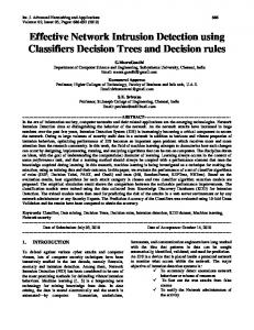
2. Anomalies and Anomaly Detectors Cyber security data can come in many forms. There is some structural commonality, though, and alignment points for possible data integration. Most of the data set can be viewed as conveying information about who did, what, to whom, and when they did it, which we refer to as a “Who-What-toWhom-When” structure. A firewall log is a good example of cyber security data. Each record of the log will be referred to as a microevent or simply event. Each event describes the activity taken by the firewall and includes: source IP address and source port that represent “Who”; destination IP address and destination port that represent “to Whom”. For each event there are firewall event codes including action (e.g. Build) and the protocol (e.g. TCP) that together identify “What”. Time, as usual, is also included and it uniquely represents “When”. An example of a sequence of firewall events is shown in Figure 1. The IP addresses are represented graphically as stars, and ports are represented as IJCNS
B. D. CZEJDO
ET AL.
595
Figure 1. Graphical representation of an example sequence of firewall events.
rectangles. Each event is represented graphically as a directional link. Time is graphically represented as a pentagon attached to the directional link and firewall event codes are represented as rounded rectangles also attached to the directional link. The analysis can be based on the individual events or on the aggregations of events. In the example, there is an event that uses the TCP protocol and destination port 6667, which could be rare since IRC chat services might be prohibited. Another example of an anomalous event would be traffic terminating at a non-DNS server on destination port 53. An example of anomalies for aggregations of events is presented in Figure 1. The occurrence of multiple “Build” events coming from the same “Who” and going to the same “to Whom” in very close time is anomalous with respect to expected network traffic flow. This case shows that in addition to analyzing individual events there is a necessity to analyze aggregations of the events. There are challenges with choosing the proper aggregations in cyber security data. The groups of events corresponding to aggregations should have appropriate size to differentiate between “typical” and “anomalous” temporal aberrations, e.g. different load for different days of the week vs. malicious events identified from the noteworthy events. With small groups, the sparsity of micro-events may be insufficiently to provide a reliable probabilistic analysis. With the larger group the probabilistic analysis will be more reliable. At the same time if the group is too large it might not properly reflect the typical temporal aberrations. As we move out to wider Copyright © 2012 SciRes.
groups, these more local effects will have reduced impact on the averages. Domain knowledge will guide the choices of the types of aggregations sought after to indicate possible known attacks. Indeed, it is easy to see that the aggregations used to find a Distributed Denial of Service attacks and a Social Engineering Phishing attacks can be at differing scales. Hence, there is a tradeoff between sparsity and specificity. Various aggregations can be used to identify anomalousness of a group of events through probabilistic computations. An aggregation is a way of collecting events into a macro-event and typically assigning some aggregate value to that macro-event, such as count. Many possible ways to aggregate events can be considered. The typical aggregations are by some attribute value, e.g. aggregating events by the same event code and source IP. Since cyber security data analysis should be very sensitive to the temporal aberrations, the time limits are typically imposed on at least some aggregations e.g. by a fixed time window or by a fixed number of events. The goal is to create a model to provide various probabilistic measures for cyber security analyst to assist him/her with maliciousness detection through various anomaly indicators as shown in Figures 2(a) and (b). One model of determining anomalousness is based on simple probabilities of occurrence of a micro- or macroevent. Unfortunately, a basic probability threshold is a poor proxy for anomalousness. We can see it clearly by considering a property with a very big domain of N values (where values have approximately the same probability and no value is ever practically repeated) and a IJCNS
596
B. D. CZEJDO
Malicious Atypical
Typical (a)
Atypical
Malicious
Typical
Atypical
Atypical
(b)
Figure 2. (a) Relationships between Typical, Atypical and Malicious for a simple anomaly analysis; (b) Relationships between Typical, Atypical and Malicious for different anomaly specifications.
property with a small domain with only two values (where only two values occur but one with the probability 1/N). We would expect the occurrence of any value for the first property to be much less anomalous than the rare value for the second property, even though both would have a probability of about 1/N. The choice of a probability threshold is directly dependent on the underlying probability distribution describing the data. There are different approaches that satisfy the general requirements for understanding of anomalousness. In our system we use the following definition to identify exceptionally rare events:
A g log P P G P g
(1)
where G is a random variable distributed according to the counts and g is one value it can take. The outer probability on the right-hand side is random with respect to G. The computation of this anomalousness is as follows. First, we compute the counts of appropriate groups of events, and then we compute probability distribution for each group P(g). Then we can compute the tail probabilities to find the anomaly for each group g. A similar approach can be used to identify exceptionally frequent events.
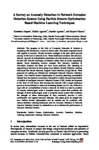
3. Cyber Security Data Warehouse A cyber security data warehouse can be built from various network data. Specifically, it can be built from the firewall data log that was described in the previous section. The data warehouse star schema for the firewall data log can be designed as shown in Figure 3. The model includes the four main components of the “WhoWhat-toWhom-When” structure as dimension tables: Source Machine, Request, Destination Machine and Time. The fact table, in our case, contains information about firewall events. The firewall events can be referred to Copyright © 2012 SciRes.
ET AL.
shortly as events. The role of each table is as follows. The Source Machine dimension contains the information for a specific machine initiating the event i.e. IP address and port used by the machine, and other attributes e.g. Machine Class. The key identifier for each object in the Source Machine dimension is the composite attribute {Source IP, Source Port}. The Request dimension contains the information about the firewall event codes that include Action (e.g. “Build”) and the Protocol (e.g. “TCP”), and other descriptions and classifications. The key identifier for each object in the Request dimension is the composite attribute {Action, Protocol}. The Destination Machine dimension has a similar structure to Source Machine and contains IP address, port used by the machine, and other attributes e.g. Machine Class. The key identifier for each object in the Destination Machine dimension is the composite attribute {Destination IP, Destination Port}. Each event has a time stamp represented by the Time dimension that can also contain some time classification e.g. part of day. The key identifier for each object in the Time dimension is the attribute {Time} which is actually a composite attribute equivalent to pair of attributes Day and Hour. The fact table, also referred as event table or simply T01, contains the log of all firewall events made from one machine to another machine at a specific time. The fact table has seven attributes: Time, Source IP, Source Port, Protocol, Action, Destination IP, and Destination Port. These attributes are foreign keys and allow to access and group events based on dimension table values. We will refer to all foreign keys as index attributes, and underline their name since other attributes can also be present in the fact table. Since each event has a time stamp, the Time attribute is actually a primary key attribute of the fact table, but the implication of this for our approach is minimal as it is discussed later.
4. Main Summarization Hierarchy for a Cyber Security Data Warehouse One of the fundamental operations for a data warehouse is the processing of the fact table in an anticipation of user queries. The new tables can be obtained by aggregation of events in the fact table and summarizing information (creating information summary) for each aggregation. These new tables are, referred to as summary tables. Summary tables in a cyber security warehouse can also contain information about event anomalies. It is important, therefore, to develop a systematic method for the design of the hierarchy of summary tables, which results in a systematic method to access anomaly information. In general, the hierarchy of summary tables can be modeled as a directed acyclic graph (DAG). Let us look IJCNS
B. D. CZEJDO
ET AL.
597
Figure 3. The initial star schema for the cyber security data warehouse.
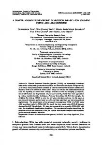
at an example of hierarchy T11, T21, ···, T71 of summary tables obtained from our fact table (T01) containing as shown in Figure 4. Level zero is for the fact table which describes all events. The first level consists of summary tables containing information about aggregations obtained from the fact table by reducing it by a single index attribute, e.g. the summary table T11 is obtained by summarizing information about all T01 events that came from the same Source Machine, had the same Request, and were directed to the same Destination Machine but happened any Time. We can consider the second level as the one consisting of summary tables containing information about aggregations obtained from the first level by reducing it by an additional index attribute. For example, the summary table T21 could be obtained by summarizing information taken from T11 for each group that came from the same Source Machine, had the same Request, and were directed to the same IP address as shown in Figure 4. We could also interpret the third level as the one consisting of summary tables containing information about aggregations obtained from the fact table by reducing it by two index attributes. In this paper, however, we concentrate on investigating the relationships between summary tables in the same or in an adjacent level. The reduce operator, referred to as R, is used to indicate what type of the grouping will be used for summarization. The R operator can be represented graphically as a label on the link between the tables e.g. from table T01 to T11. The first argument for the R operator is an index attribute, e.g. Time. It determines what index attribute will be dropped in the newly created summary table. The second argument for the R operator is the Copyright © 2012 SciRes.
grouping method. For the main summary graph only the simple grouping method based on removing one index attribute will be allowed. This simple grouping method is denoted as “index based”. In general, the number of summarization levels in the summarization graph is equal to the number of index attributes and the number of summary tables on each level can be computed based on all possible combinations for the corresponding subset of index attributes. In our case, we have 7 levels and on the highest level there is single table T71 that contains the maximum summarization—the summarization on the highest abstract level. The directed links are showing possible transformations from one table to another. The levels of the summarization graph correspond to various granularities for grouping. The first summarization level corresponds to the least coarse (finest) grouping, the next (second) summarization level corresponds to coarser grouping, etc. There are seven levels of granularity for our data warehouse. At level 0 (lowest level), the granularity is the finest and the records of actual events are stored. When these records are summarized, the level of granularity is coarser. For example T11, a time independent summary table, has the coarser granularity. Furthermore, T21, T31, etc. are even coarser. In general, coarser levels of granularity provide fewer details but require smaller records to be stored. In practice, some nodes in the graph are of a lesser importance. Since the Time attribute is a primary key attribute for the fact table T01, the first summarization level practically has only one meaningful table T11. Applying the R operator with any argument other than Time argument would not perform any grouping, but rather it IJCNS
598
B. D. CZEJDO
ET AL.
Figure 4. The main summarization hierarchy for the cyber security data warehouse.
would project one of the attributes from the T01 table. The steps described above can also result in new attributes for each table. These attributes describe the properties of newly created groups. Each group can have various properties assigned to it, e.g. Count property can store the number of events. In our example of the summary table T11, the Count property is computed by simply counting the number of events in each group. Let us describe summary tables and their attributes more forCopyright © 2012 SciRes.
mally. Each summary table contains a set of groupings G g1 , , g i , , g n where each group gi needs to have some properties computed and stored as table attributes. The number of groups is determined by possible values of the summary table index attributes. The R operator specifies how each grouping gi is created. The computation of the property is determined by a computation method. The “Count” computation method allows to compute values of the Count property by simply countIJCNS
B. D. CZEJDO
ing the number of events in each group gi. The “Sum” computation method allows to compute values of the CountAll attribute by adding count property for each group gi. This is equivalent to counting all events in the fact table. It is important to notice that the summary table does store the actual sequence of events (or sequence of sequences of events, etc.) but rather it stores an information summary for an implicit group of events (identified by its index attributes). This information summary is stored in the form of each group’s properties. There are other computation methods, e.g. based on attribute values of the same table. The Probability is a good example of such property. The unconditional probability pi can be computed for each group gi and stored as its non-index attribute probability. For the cyber security applications it is also important to compute various conditional probabilities (if summarization level allows for that) for each aggregation gi and stored as its non-index attributes probabilityC1, probabilityC2, etc. The Anomaly attributes can be computed based on the formula discussed in Section 2. In a typical situation the computation of anomaly is based on attribute values of the same table. The anomaly is computed for each group gi based on distribution of the values of the attribute probability. Actually, the anomalies for low and high values can be computed and stored as its non-key attribute as anomalyLow and anomalyHigh. Additionally, the anomalies for low and high values can be computed for each aggregation gi based on conditional probability distributions and stored as its non-key attribute anomalyC1, anomalyC2, … To simplify our presentation we will assume that all these anomalies are represented by a single anomaly property. The different tables have different anomaly indicators. The granularity of the tables corresponds to the granularity of anomalies. Since the anomalies of networking events are related to some aggregation of events the granularity of anomaly on the zero level is often considered to be too fine. When anomalies are computed on summarized data the results are more likely to point to noteworthy aggregations. For example T41, a time independent summary table, can show a significant atypical behavior.
5. Complex Aggregation Tables for Event Windows So far we have discussed the main hierarchy graph with its main summary tables using nodes and simple reductions (by one index attribute) as directed links. In the case of network traffic data, anomalies are often not rare objects, but unexpected bursts in events. Thus anomaly requires not only a probabilistic definition of atypical objects, but also appropriate probabilistic computations Copyright © 2012 SciRes.
ET AL.
599
for aggregations of network events. In this section we present data models for bursts of the events and techniques to identify anomalies in the bursts of the events. Generally the aggregation method to model bursts of events can be window based or event proximity based. In this paper, we address only window based aggregation. Here, we have different types of windows with two most obvious: fixed-time window and fixed-number-of-events window. Let us concentrate on fixed-number-of-events window. We can model a sliding fixed-number-of-events window by proper aggregation of event (fact) table T01. The previously discussed R operator needs to be extended to denote this aggregation properly. The extension is based on an observation that a simple index based aggregation would not suffice here, but more complex aggregation of events should be here performed, i.e., aggregation of all events within the window. Additionally, each window needs to be uniquely identified since we want to perform various window based computations. The beginning or ending time of window can be used for that purpose. We will denote the operator to perform window based aggregation as R({}, fixed-number-of-events-window). There is an empty set as a first argument of R since the Time index is kept even though it needs different interpretation. The second argument fixed-number-of-eventswindow indicates the type of complex aggregation. Other types of aggregation can also be used, e.g. fixed-timewindow. Deciding about the overlap of sliding windows requires some attention since it will affect the number of aggregations. The extreme case of associating a window with each event is not practical because of the large amount of computations and data (no data reduction), while single events would not affect the total count that much. Another extreme case of making window disjoint is not sufficient since the burst of events divided into two windows might not trigger the anomaly detector. Practically, some overlapping factor needs to be selected, e.g. 50%. As a result the data contain many redundancies since the same event will be present in many groupings. For the window overlapping factor of 50%, the replication factor will be close to 2. The information about window based aggregations can be stored in a summary table, e.g. the new table T01A1. This new table does not belong to main summarization hierarchy since complex aggregation was used. It will be placed in the new layer of the node T01 since it uses the same index attributes. In general, any newly introduced complex aggregation will result in the creation of the new table and new layer of the summarization hierarchy. The new table is placed in that layer in the same node as the main summary table with the same index attributes. The new table, in our case was named T01A1 since “A1” IJCNS
600
B. D. CZEJDO
will stand for additional layer number one related to the additional complex aggregation. The newly created table can be a starting node of a new hierarchy placed in the new layer. Other tables of the new hierarchy would also correspond to main summary tables that have the same index attributes. For example, data in table T00A1 can be summarized into another table T11A1 by the R operator with the simple aggregation i.e. R(Time, index-based). The table T21A1 will also belong to the same layer since the simple aggregation was used. In general, any new table constructed by a simple aggregation will belong to a layer of the initial table. The relationships between tables in the different layers of the same node can be identified. For example the table T11A1 can be very similar to T11 after adjusting for event redundancies by, e.g., dividing count by 2 when windows are overlapping by 50%. The summarization hierarchy will, therefore, consists of a main layer, called also layer number zero or main hierarchy and additional layers corresponding to other aggregation methods or derived hierarchies. The aggregations’ properties can be computed using different computation methods as before. Let G g1 , , g i , , g n be a set of aggregations (groups) stored in table T00A1 where each aggregation gi consists of network events in a fixed size window. We will use again our basic probabilistic model for computing anomalies: count of events of the same type in each window (counti), compute the probabilities for each aggregation (events of the same type), and then compute the anomalies for each aggregation based on the probability distribution of P(G).
6. Using Summarization Hierarchy for Situational Understanding of Cyber Security System We implemented our cyber-security data warehouse model on the IEEE Vast 2012 Situational Understanding and Cyber-forensics data [14]. The summarization hierarchy graph was created based on the previously defined index attributes: Time, Source IP, Source Port, Action, Protocol, Destination IP, and Destination Port. We used mostly the layer of the summarization hierarchy corresponding to window based aggregations. These aggregations were constructed for non-overlapping windows with the five minutes window duration. First, the anomalous behavior with respect to the volume of all traffic was detected based on the appropriate table on the sixth level of aggregation (called table T62A4) with the single index attribute Time indicating the beginning of the window, and non-index attribute Count describing the traffic volume. Using this grouping, we were able to determine that the network traffic was Copyright © 2012 SciRes.
ET AL.
Figure 5. The additional layer of complex summary tables for the window based aggregations.
anomalous (drastically lower) for many windows. More specifically we could identify a four-hour period of anomalous traffic. This anomaly was a starting point of a down traversal (drill-down operation) of the summarization graph. We looked at the lower level (level 5) aggregation described by a table (called table T52A4) with two index attributes Time and Action, and non-index attribute Count describing the traffic volume. We observed an anomalous high percentage of traffic through the firewall that was related to the value “system log entry” of the attribute Action. The discovery of these anomalous events was very important. The system log entries indicated that the connections were made to the firewall itself and that changes were made to the firewall settings. It looked like dangerous tampering to firewall information that may have contributed to other traffic deviations around the same time. Another anomaly was discovered by traversing the part of the summarization graph containing tables on the fourth and lower aggregation level with at least three index attributes Time (indicating the beginning of the IJCNS
B. D. CZEJDO
window), Source IP and Destination IP. This traversal resulted in the observation that exactly one source IP was responsible for all traffic from workstations to websites for some specific window sequences. This strongly indicated a possible misdirection or man-in-the-middle attack where all traffic is routed through an intermediate contact. Yet another anomaly was discovered by applying complex aggregation to the attributes Machine Class for both source machine and destination machine. The aggregation resulted in the summary table (called table T62A5) with the original index attribute Time uniquely identifying each window and three new attributes Source Computer Class, Destination Computer Class, and Count. Indeed, by considering the collection of events partitioned by computer class, we observed the deviation from the typical traffic pattern originating from the DNS server and ending at DNS servers. Actually, for the IEEE Vast 2012 data, the anomalous behavior was observed after the first 20 hours. Departure from this baseline indicated a misdirection of routing, possibly involving serious exfiltration of protected data.
7. System Architecture The conceptual system architecture is shown in Figure 6. It is built based on typical data warehouse architecture and contains two main components: Cyber Security Data
ET AL.
601
Warehouse and Cyber Security Event Database. Both components use the aggregation hierarchy graph as a model for the data storage. The Update Data Warehouse processor updates Cyber Security Data Warehouse periodically (e.g. daily) with recorded events that occurred after the last update from the Cyber Security Event Database. In addition, there are Anomaly Global Patterns, and Anomaly Occurrence databases. Anomaly Global Patterns are updated periodically at the same time the data warehouse is updated. Anomaly Global Patterns are computed based on values of the anomaly attributes in the aggregation hierarchy graph. The simple interpretation of the content of Anomaly Global Patterns is that patterns contain all historical event probability distributions (Layer 0, 1). The simple interpretation of the Cyber Security Event Database is that it contains the current events in the form of the most recent window (Layer 1). The Identify Anomaly processor is a crucial component of the system and works on-line to compute anomalies in the current event table T11 and in the tables above based on historical event table T11 practically updating the Anomaly Occurrences database (actually a part of Cyber Security Event Database). There are two main tasks for Anomaly Integration and Visualization processor. First, it combines the anomalies into a single measure and displays the result as a warning meter. Second, it displays the individual anomalies for the cyber security analyst.
Figure 6. System architecture. Copyright © 2012 SciRes.
IJCNS
602
B. D. CZEJDO
The cyber security analyst can specify globally and for each node the threshold for anomalies to be displayed. The cyber security analyst can also define new nodes in the graph by associating the new aggregation with it.
8. Conclusion In this paper, we introduced the generalization of aggregation operation as applied to a cyber security system. We discussed the concept of an event aggregation graph that contains not only information about various aggregations but also anomalies related with each aggregation level. The aggregation graph once implemented can be explored to enhance the cyber security analyst’s situational understanding. When the graph is presented to the cyber security analyst, only the relevant nodes are included, allowing him/her to focus on most probable threats of network intrusion.
REFERENCES [1]
[2]
[3]
[4]
H. Kriegel, P. Kröger and A. Zimek, “Outlier Detection Techniques,” Proceedings of 13th Pacific-Asia Conference on Knowledge Discovery and Data Mining (PAKDD 2009), Bangkok, Thailand, 2009. http://www.dbs.ifi.lmu.de/Publikationen/Papers V. Chandola, A. Banerjee and V. Kumar, “Anomaly Detection: A Survey,” ACM Computing Surveys, Vol. 41, No. 3, 2009, Article 15. S. Axelsson, “The Base-Rate Fallacy and the Difficulty of Intrusion Detection,” ACM Transactions on Information and System Security (TISSEC), Vol. 3, No. 3, 2000, pp. 186-205. doi:10.1145/357830.357849 H. Teng, K. Chen and S. Lu, “Adaptive Real-Time Anomaly Detection Using Inductively Generated Sequential Patterns,” Proceedings of IEEE Symposium on Security
Copyright © 2012 SciRes.
ET AL. and Privacy, Marlboro, 7-9 May 1990, pp. 278-284. doi:10.1109/RISP.1990.63857 [5]
D. Denning, “An Intrusion Detection Model,” Proceedings of the Seventh IEEE Symposium on Security and Privacy, 7-9 May 1986, pp. 119-131.
[6]
A. Jones and R. Sielken, “Computer System Intrusion Detection: A Survey,” Technical Report, Department of Computer Science, University of Virginia, Charlottesville, 1999.
[7]
S. Cho, “Incorporating Soft Computing Techniques into a Probabilistic Intrusion Detection System,” IEEE Transactions on Systems, Man, and Cybernetics, Vol. 32, No. 2, 2002, pp. 154-160.
[8]
A. Venturini, “Time Series Outlier Detection: A New Non Parametric Methodology (Washer),” Statistica—Università di Bologna, Vol. 71, 2011, pp. 329-344.
[9]
E. M. Ferragut, D. M. Darmon, C. A. Shue and S. Kelley, “Automatic Construction of Anomaly Detectors from Graphical Models,” Proceedings of IEEE Symposium on Computational Intelligence in Cyber Security (CICS), Oak Ridge, 11-15 April 2011, pp. 9-16. doi:10.1109/CICYBS.2011.5949386
[10] A. Gupta, V. Harinarayan and D. Quass, “AggregateQuery Processing in Data Warehousing Environments,” Proceedings of the VLDB, Zurich, 11-15 September 1995. [11] J. Bischoff and T. Alexander, “Data Warehouse: Practical Advice from the Experts,” Prentice-Hall, Upper Saddle River, 1997. [12] J. Widom, “Research Problems in Data Warehousing,” Proceedings of the 4th International Conference on Information and Knowledge Management, Baltimore, 28 November-2 December 1995. [13] B. Czejdo, M. Taylor and C. Putonti, “Summary Tables in Data Warehouses,” Proceedings of ADVIS’2000, Turkey, 25-27 October 2000. [14] http://www.vacommunity.org/VAST+Challenge+2012
IJCNS