Network modelling applied to CORE power transformers and

International Colloquium Transformer Research and Asset Management Dubrovnik, Croatia, May 16 – 18, 2012 Hugo M. R. Campelo EFACEC Energia, S.A. [email protected]

Carlos M. Fonte FEUP University of Porto [email protected]

Ricardo C. Lopes EFACEC Energia, S.A. [email protected]

Madalena M. Dias FEUP University of Porto [email protected]

José Carlos B. Lopes FEUP University of Porto [email protected]

Network modelling applied to CORE power transformers and validation with CFD simulations SUMMARY Parametric studies, based on Computational Fluid Dynamics (CFD) simulations, have been made to evaluate the influence of geometrical configuration and operating conditions on the friction factor and heat transfer coefficients. New correlations for the friction factor and heat transfer coefficients have been developed for better description of flow and temperature distribution. A computational tool coupling the Thermal-Hydraulic Network Models (THNMs) concept with CFD calibration has been developed – named FluCORE. This tool estimates the steady-state temperatures under natural (ON) and forced (OD) cooling regimes with comparable results to CFD simulations. FluCORE is a lumped parameter model and has been found to be an industrializable and versatile decision helper, capable of being adjusted to different operating conditions and design configurations while reducing considerably the computational time and effort of simulation when compared to CFD simulations. Key words: Power transformer, disc-type windings, CFD, thermal network models, hot-spot

1.

INTRODUCTION

The lifetime of every power transformer depends largely on the temperature of its insulation and the common cellulosic-based insulating parts of its windings are typically the most thermal stressed structures. These polymeric entities experience a progressive degradation within operation conditions as its chemical bonds break. The temperature field is definitely influencing this chemical reaction and the maximum temperature (hot-spot) is the limiting step. As a result, the heat generated inside power transformers is removed by circulating a cooling fluid, typically mineral oil, through a complex set of interconnected ducts. The geometrical configuration of the ducts determines the oil flow distribution along the transformer, which affects the heat removal efficiency and the position and magnitude of hot-spots.

1

To avoid experimental verification each time a new power transformer is designed, manufacturers often resort to mathematical models to ensure the control of temperature inside the power transformer, including the magnitude and position of hot-spots and average temperatures of the oil and conductor discs at different positions. Two methods may be used to model the cooling of a power transformer, CFD and THNM. CFD is a powerful tool for the simulation of flow and heat transfer. Several studies have been performed for the development of CFD models applied to power transformers and although detailed studies are possible, this is a fairly complex and time consuming method [1, 2]. The THNM concept implies a division of the spatial domain into a network of smaller and simplified elements. The global model comprises two separate models: the hydraulic model; and the thermal model. The hydraulic model describes the oil flow distribution through the network of ducts and junctions. The flow through the network is modeled using the analogy with an equivalent electric circuit where the flowrate through the ducts and the pressure drop correspond to the electrical current across the resistance branches and to the voltage between nodes, respectively. The heating of the oil throughout the coils due to energy dissipation on the discs is solved by coupling the thermal model that includes all the heat transfer mechanisms, with the hydraulic model. Early models have been built in a very simplified way by considering constant cross-sectional area on the radial ducts. The axis-symmetrical cylindrical geometry of the power transformer is approximated to rectangular ducts with constant cross-sectional area [3, 4]. These models also consider that the oil flows in defined paths and local circulations are ignored and the wall temperature at each surface of the conductor disc is assumed to be constant [4, 5]. More sophisticated models [2, 6, 7] take into consideration the variation of temperature along the radial and axial directions and give importance to minor losses that actually have dominant influence on the flow distribution and pressure loss. These works use empirical correlations for the friction factor and heat transfer coefficients relying solely on isolated experimental measurements or indirect measurements to validate the simulation results. Herein a new numerical approach based on THNM is proposed to predict the temperatures inside core type power transformers.

2.

CORE TRANSFORMER GEOMETRY

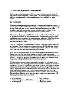
A core type power transformer comprises a magnetic iron core surrounded by different kind of windings. These windings consist on a conductor wire usually made of insulated copper placed concentrically along the axial direction of the power transformer, forming conductor discs. In this work, a core type power transformer design (25 MVA – ODAF - 45/16/5 kV – Ynyn, 50 Hz, 3 phases) has been studied. For each phase, vertical and radial positioned obstacles (sticks and key spacers, respectively) divide the transformer into 12 sections. Since these sections are identical, each section can be considered as a repetitive slice, and used for simultaneous flow and heat transfer modelling simulations, Figure 1. Each phase involves four windings, Figure 2: two disc type windings, Low Voltage (LV) and High Voltage (HV); and two layer type windings, Tertiary (T) and Regulation (Reg). In the case of the LV and HV windings, the conductor discs are placed horizontally in layers separated by spacers, originating ducts, where the cooling oil flows radially. As a way to direct the flow throughout these radial ducts, washers are inserted periodically along the vertical direction to impose a zigzag flow through the windings. The set of discs and corresponding ducts separated by two washers is referred as a block. The T winding discs are not separated by spacers, hence forming a single layer. The Reg winding is a hybrid winding with sections where the discs are separated by spacers, and sections where the discs form a single layer.

2

Figure 1 – Isometric view of CORE transformer phase, 12 identical sections, showing the half-section symmetry. 3.

CFD SIMULATION

3.1.

2D and 3D Computational Grids

Figure 2 – Cut view of 4 windings of a single phase.

Core power transformers have a cylindrical shape, but the geometry of the flow and copper domains is not strictly axisymmetric. This caused by the solid spacers that are positioned vertically to separate the different sections, or radially (key spacers) creating the internal oil cooling ducts. These spacers hamper the heat transfer and increase friction at the walls. These factors cannot be directly taken into account in a simplified 2D radial axisymmetric simulation. A 2D computational conformal grid with 800 000 elements of variable size has been created, using a more refined grid in critical zones with the smallest element size of 0.7 mm – Figure 3a. This grid has been subjected to several sensitivity tests and it has been found to be the one with the best precision/computational effort ratio. In order to access the full transport details a 3D simulation model has been created, representing the smallest repetitive section of the transformer (volume limited by two vertical planes as shown in Figure 1). For the 3D simulation, a tetrahedral/hexahedral hybrid mesh with 2 450 000 elements has been created. The mesh size is in average 2.5 mm, although in critical zones, the mesh refinement is 0.7 mm – Figure 3b.

(a) (b) Figure 3 – Computational grid sample for the a) 2D and b) 3D CFD models 3

3.2.

Physical Model

Steady-state governing equations: continuity (Equation 1), momentum (Equation 2) and energy (Equation 3) for a Newtonian fluid motion:


∇ ⋅ ( ρυ ) = 0,

(1)





∇ ⋅ ( ρυ × υ ) = −∇p + µ ( ∇ 2υ ) + g ( ρ − ρ ref ) ,

(2)


∇ ⋅ ( ρ c pυ T ) = ∇ ( k ∇T ) .

(3)

Conduction equation in the solid copper and insulation paper:

∇ ( k ∇T ) = S E , where

3.3.

(4)

S E accounts for the electric current heat dissipation distribution into the copper. Material Properties

The oil density temperature dependence is:

ρ = 868 (1 − 6.40 × 10−4 (T − 293) ) ,

(5)

-3

where ρ is the naphtenic oil density in kg m at temperature T in K . The oil viscosity temperature dependence has been obtained experimentally using a cone/plate rheometer within the temperature range of 20°C to 80°C :

 3.48 ×103  , T  

µ = 1.43 ×10−7 exp 

(6)

where µ is the viscosity of the oil in Pa ⋅ s and T is the temperature in K . Within this range of temperature, viscosity varies by one order of magnitude. The oil thermal conductivity and heat capacity have been assumed constant since its variation is negligible within the studied temperature range:

c p = 2.02 kJ kg -1 K -1 and koil = 0.126 W m -1 K -1 , respectively. A simulation that takes into account the individual insulated conductors inside the disc would require a large computational effort. For this reason, the total disc volume has been considered a homogeneous medium where an equivalent orthotropic thermal conductivity is calculated in the radial, axial and azimuthal directions, including the contribution of copper and insulation paper in all directions. The conduction model has been validated in a previous work [8] and with maximum temperature deviations of 10% when comparing the real simulated geometry to the simplified conduction model. Table I – Orthotropic conductivities (W.m-1.K-1) used in the main windings (LV and HV). Thermal Conductivity Direction Tangential Axial Radial 3.4.

LV 389 3.90 0.90

HV 389 287 0.60

Boundary Conditions

The hydrodynamics and thermal boundary conditions used in the CFD simulations (2D and 3D) are summarized in Table II. The inlet boundary conditions have been defined in order to ensure an oil 3

flowrate of 37.4 m h at 80°C . In both simulations power dissipated by each winding has been uniformly dividided by each disc, neglecting for this purposes the non-uniform heat distribution induced by the magnetic field. 4

Table II – Boundary conditions and heat sources for 2D/3D CFD simulations. Inlets

3.4.

Pstatic = 248 Pa (2D) and Pstatic = 310 Pa (3D) Tinlet = 80°C

Outlets

Pstatic = 0 Pa

Solid walls

No-splip condition

Magnetic core walls

Tcore = 100°C

Windings and core heat source dissipations

HV LV T REG CORE

344 kW/m3 313 kW/m3 4.33 kW/m3 413 kW/m3

(48.4 kW total) (31.3 kW total) ( 90 W total) (7.93 kW total) (4.38 kW total)

Simulation Results

Figure 4 shows the oil streamlines in several locations inside the windings of power transformer under study. The streamlines over a block between two consecutive washers, Figure 4a, shows the existence of vortex-type structures at the entrance region of the radial ducts that enhance the friction factor in this particular region. There are some vortex structures also at the exit of Reg winding, Figure 4c. However, the flow is typically bi-dimensional and laminar, having a typical Reynolds number lower than 1200.

(b)

(a) (c) Figure 4 – Flow streamline maps a) between washers, b) at the entrance of the T winding and c) at the outlet of the HV and REG windings obtained with the 2D CFD model. Figure 5 depicts the radial oil velocity profile along the height (2D model). It exhibits a typical ‘Ushaped’ profile with the minimum velocity in the middle disc of each block. Negative radial velocities represent flow away from the transformer core. The velocity patterns in each block limited by two washers are very similar. The radial ducts near a washer present higher velocity values, with the highest values observed right before each washer (Figure 5a). These higher velocities promote better heat transfer rate,

5

reflected in the lower temperatures observed in these zones (Figure 5b). For the simulated configuration, the HV winding presents higher local temperatures when compared with the LV winding. The averaged oil temperature for all 4 windings is 82.9ºC with an outlet temperature of 85.7ºC.

(a)

(b)

Figure 5 – a) Radial velocity and b) Temperature profiles as function of height obtained with the 2D model. The temperature fields in 2D and 3D have a similar trend (Figure 6), but the 3D temperatures are always slightly higher as the effective heat transfer area is lower mainly due to the presence of key spacers.

(a)

(b)

Figure 6 – Temperature distribution contour maps for a) 2D and b) 3D model.

6

The overall hot-spot is located in the HV winding with a value of 112.4ºC for the 2D simulation and 114.9ºC for the 3D simulation. Table III shows the simulated average and hot-spot temperatures of the two most significant windings (HV and LV). Table III – Simulated temperature in the two most important windings for the ODAF cooled transformer. Winding Avg. Temp. (ºC) Hot-Spot Temp. (ºC) Avg. Temp. (ºC) Avg. Grad. (ºC)

HV LV

2D Simulation 99.6 112.4 98.6 15.7

3D Simulation 102.4 114.9 102.3 19.4

The computed temperature parameters, from 2D and 3D simulations, differ in a maximum of 3.7°C. These results, and also similar outcomes from simulations at different operating conditions, revealed that the extra degree of computational effort with 3D effects is not necessary within a predictable relative maximum deviation (2D/3D) around 4%.

4.

THNM SIMULATION

THNM approach enabled the development of a lumped parameter thermal tool named FluCORE. Alternatively to CFD, which is a distributed parameter approach where the equations governing the transport phenomena result in complex systems of partial differential equations, the developed tool subdivides the space in discrete points being the transport phenomena governed locally by simple algebraic equations sets, and the consequent time-to-solution is found to be considerably shorter. In these algebraic equations systems, there is still need for some transfer coefficients data, namely friction factors and heat transfer coefficients correlations that have been obtained from systematic analysis of the 2D CFD model previously described. The global model comprises a hydraulic network model, HNM, and a thermal network model, TNM. FluCORE manages these two coupled models in an iterated fashion, Figure 7, in order to achieve the final steady-state temperature and velocity fields inside the windings of a core type power transformer

Tin ,qin Hydraulic Network Model (Isothermal Simulation at Tin )

q*(k) Estimative Th,Tv,Tc

q (k) Thermal Network Model

Hydraulic Network Model (Non-Isothermal Simulation at Tin )

IF NOT CONVERGED

q (k), Th(k), Tv(k), Tc (k)

Figure 7 – Block diagram depicting the coupling method between hydraulic and thermal networks models.

7

4.1.

HNM – Hydraulic Network Model

After establishing an electrical-hydraulic analogy and apply it to the discrete points of the domain under study, as shown in Figure 8 it is possible to re-write the two Kirchhoff laws (Equations 7 and 8) in hydraulic terms as follows :

[ qk + qk +1 ] − [ qk + 2 + qk +3 ] = 0 where

q is the volumetric oil flow rate at the nodes, b

rad

[ pk − pk + 2 ] + [ pk + 2 − pk + 3 ] and

(7)

c

rad

− [ pk +1 − pk + 3 ] − [ pk − pk +1 ]

=0

(8)

p is the local node static pressure.

(a)

(b)

Figure 8 – a) flow network description and b) electrical analog. As depicted in Figure 8b the pressure drop between each node is modeled, Equation 9, using a resistive element due to friction and a source term due to velocity variations and/buoyancy effects particularly significant under ON conditions:

∆Pk = Rk qk + ∆Pks .

(9)

The resistive elements are described using different equations whether it is a radial duct , Equation 10: k rad

R

1 M −1 = ∑ ρ Thmk ,m f rad Re Thmk ,m 2 m =1

(

) ( (

))

 Lr  qk − 2 − qk rad Dh ,k ,m [ M − 1]  Akrad ρ Thmk ,m  ,m

where M is the number of nodes in which the radial duct is subdivided, local temperature, T

h ,m

(

ρ

)

 ,  

(10)

is oil density dependent on

, the average temperature between two consecutive nodes, f rad is the radial

friction factor correlation extracted from CFD simulations, Lr is total length of the radial duct, Dh is the local hydraulic diameter, as

Akrad , m is the local flow section area, and finally the local Reynolds number defined

Re = ρ Dhυ µ , where µ is the oil viscosity at local temperature, and υ is the local average velocity

in the duct. For the axial duct, the ducts are further subdivided whether the flow is converging (confluence) or diverging (branching), Equations 11 and 12:

8

b,k axi

R

( ( )) H ( ) D

b f axi Re Tvmk ,0 1 = ρ Tvmk ,0 2 2

L −1 1 b + ∑ ρ Tvmk ,l f axi Re Tvmk ,l l =1 2

) ( (

(

( ( )

b f axi Re Tvmk ,L 1 + ρ Tvmk ,L 2 2

(

 /2 qk    Aaxi  T ρ vmk ,0  f ,k  H disc ,k +1 [ L − 1]  qk  axi axi  Dh ,k A ρ Tvmk ,l  f ,k spacer , k axi h,k

))

(

)

(

)) H

spacer , k + 2 axi h,k

D

2 qk  axi  Af ,k ρ Tvm k ,L 

(

)

)

   

(11)

 .  

This resistive expression for the axial branching ducts is identical excepting that L now represents the number of nodes in which the axial duct are subdivided, Tvm is the average oil temperature between two consecutive vertical nodes, H represents the height of the spacer or of the disc and f axi is another axial branching friction factor correlation also extracted from CFD simulations. c ,k axi

R

( ( )) H

c f axi Re Tvmk ,0 1 = ρ Tvmk ,0 2 2

(

L −1

)

1 c + ∑ ρ Tvmk ,l f axi Re Tvmk ,l l =1 2

(

) ( (

))

( (

)) H

c f axi Re Tvmk ,L 1 + ρ Tvmk ,L 2 2

(

)

 /2 qk    Aaxi D ρ Tvmk ,0   f ,k  H disc ,k +1 [ L − 1]  qk  axi axi  Af ,k ρ Tvm Dh ,k k ,l  spacer , k axi h,k

(

)

(

spacer , k + 2 axi h ,k

D

2 qk  axi  Af , k ρ Tvm k ,L 

(

)

)

   

(12)

 .  

The resistive expression for the axial confluence ducts is identical to previous one excepting for the friction factor correlation. The axial and radial source terms are modeled using Equations 13 and 14, respectively. 2 2      T + T qk − 2 qk 1  mk −2  mk   s     ∆Paxi = − ρ  − axi    axi 2  2    Af ,k − 2 ρ Tmk −2   Af ,k ρ Tmk ,0     2 2      qk qk + 2 1  Tmk + Tmk +2     −  , − ρ    axi axi 2  2    Af ,k ρ Tmk   Af ,k + 2 ρ Tmk +2    

(

( )

( )

)

(

(13)

)

and:

9

S rad

∆P

 q 1  = − ρ Tvmk −2   axi k − 2 2   Af ,k − 2 ρ Tvmk −2 

(

)

(

2

)

  q −q   −  radk − 2 k    Af ,k ,1 ρ(Thmk ,0 )    

 qk − 2 − qk 1  − ∑ ρ Thmk ,m   rad m =1 2   Af ,k ,m ρ Thmk ,m  M −1

(

)

(

 qk − 2 − qk 1  − ρ Tvmk +1   rad 2   Af ,k , M ρ Thmk ,M 

(

)

(

The form of the axial friction factor,

  −  

2

)

  qk − 2 − qk  − rad   Af ,k , m +1 ρ Thm k ,m +1  

(

2

)

2

  qk +1  − axi   Af ,k +1 ρ Tvm k +1  

(

)

   

2

)

   

2

  −  

(14)

  .  

f axi , correlation (Equation 15) and radial friction factor,

f rad , correlation (Equation 16) are shown below. The curves have been correlated with 2D CFD data: f axi

where

 A  Re B ; Re < 194 = , C  ; Re ≥ 194  Re D

A, B, C , D are correlation constants and Re is the local node Reynolds number, and:

f rad = where

(15)

96 1 + ELr F S G  , Re 

(16)

Lr is total length of the radial duct, E , F , G are correlation constants, and S is the duct shape

factor. 4.2.

TNM – Thermal Network Model

To model the heat transfer to the oil due to the energy dissipation on the windings is necessary to solve simultaneously the equations of heat transfer within each region: • • •

Heat conduction inside the discs, Convection/conduction from the discs to the oil, Convection/conduction in the oil.

Each single disc is divided into M control volumes where the heat transfer equations are applied, Figure 9. The disc body has been considered a homogeneous medium where an equivalent thermal resistance is calculated in the radial and axial directions including the contribution of each individual component (copper and insulation paper). The heat flux values on the interface disc/oil are used as boundary conditions for the heat transfer in the oil and are placed in the geometrical boundaries of the disc.

10

Th(k+2,2)

Th(k+2,1)

Th(k+2,m)

Thm(k+2,1)

Th(k+2,m+1) Thm(k+2,m)

Tv(k,3) = Tv(k+2,0) …

…

Tc(k,1,3)

Tc(k,m,3)

Tv(k,2) … Tvm(k,1)

Tc(k,0,2)

Tc(k,2,2)

Tc(k,1,2)

Tc(k,m,2)

Tc(k,m-1,2)

Tv(k,1)

Tc(k,m,1)

Tc(k,1,1) Tv(k,0)

Tc(k,m+1,2)

…

… Thm(k,m)

Thm(k,1) Th(k,2)

Th(k,1)

Th(k,m)

Th(k,m+1) Δr

Figure 9 – Discretization of the disc region for the thermal network model. When heat conduction occurs in the central zone of the winding, Figure 9, an equivalent thermal conductivity has been considered in the radial direction, K cr , and in the axial direction, K cx and the equation of heat transfer inside the disc has been defined as:

  2 K cx K p Qgk V pk =   Ax ,m Tck ,m ,2 − Tck ,m ,3   K p H disc ,k + 2 K cx l p    2 K cx K p +  Ax ,m Tck ,m ,2 − Tck ,m ,1   K p H disc ,k + 2 K cxl p  +

(17)

2 K cr Ar ,m Tck ,m ,2 − Tck ,m−1,2 

∆r 2 K cr Ar ,m +1 Tck ,m ,2 − Tck ,m+1,2  , + ∆r

where Qg k is the local heat dissipated in the disc at node k , V pk is volume of each discretization volume partition of the disc, Tc is the local disc temperature, Ax is the heat transfer section area in the axial direction, Ar is the heat transfer area in the radial direction, paper, K p is the thermal conductivity of the paper and

l p is the thickness of the disc insulating

∆r is the radial length of each discretization

partition of the disc. In the disc surface the heat transfer is determined by a local heat transfer coefficient. The heat transferred from the disc to the inferior duct (flux A2 in Figure11) had been modeled as follows:

  2 K cx K p   Tck ,m ,2 − Tck ,m ,1  = ho ,k , m Tck ,m ,1 − Thmk ,m  ,  K p H disc ,k + 2 K cxl p  where

(18)

H disc is the height of the disc and ho is the oil heat transfer convective coefficient.

11

B2

C2

D2 A2

Figure 11 – Heat transfer in the vicinity of the windings The heat transferred from each disc surface to the superior duct (flux B2 in Figure 11), to the branching axial duct (flux C2 in Figure 11) and confluence axial duct (flux D2 in Figure 11) have been modeled with similar algebraic expressions. The heat convection within the oil has been modeled by establishing enthalpic balances between nodes. Different expressions had been used depending on the relative node position around the winding discs, as depicted in Figure 12 (A3, B3 and C3).

Figure 12 – Heat transfer in the oil. The convective heat transfer in the axial ducts (A3 flux in Figure 12) has been defined as:

[ qk − 2 − qk ] c pTh

k ,m

= [ qk − 2 − qk ] c pThk ,m+1 + ho,k ,m Ax ,k ,m Tck ,m ,1 − Thmk ,1  + ho, k ,m Ax ,k − 2, m Tck −2,m ,3 − Thmk ,m  , (19)

where

c p is the oil heat capacity at constant pressure, the convective heat transfer in the radial ducts (B3

flux in Figure 12) is defined as:

qk +1c pTvk +1,1 = qk +1c pTvk +1,2 + ho,k ,m Ar , k , M Tck ,M ,2 − Tvmk +1,1  ,

(20)

and the convective heat transfer in the confluence joints (C3 flux in Figure 12) has been defined as

qk +1c pTvk +1,0 = [ qk + 2 − qk ] c pThmk ,M + qk −1c pTvk −1,2 . The oil heat transfer convective coefficient,

ho , is computed from the Nusselt number, defined as:

Nu = where

(21)

h0 ⋅ L , ko

(22)

L is the total radial length of the duct and ko is the oil thermal conductivity. The necessary Nusselt

number correlations have been developed following a methodology proposed by Zhang & Xianquo [7], and expressed a function of the dimensionless thermal entrance length, xad , and having the general form for the radial ducts:

 1 Nu = Nu∞ ⋅  1 + b  a ⋅ xad

 , 

(23)

12

where

Nu∞ is the minimum Nusselt observed in the radial duct, or bulk Nusselt, and a and b are

correlation constants. On the other hand the Nusselt number correlation for axial ducts is quite different. This behavior is expected due to its fundamental difference in the boundaries. The axial ducts are heated only from one side, and the Nusselt number depends on the thermal entrance length as: d Nu axi = c xad

(24)

where c and d are correlation constants. For the radial and axial ducts, the Nusselt number has been fitted to CFD simulation data, similarly to the friction factor correlation curves. 5.

CFD VERSUS FLUCORE COMPARISON 3

A simulation with FluCORE has been run for an inlet flowrate of 32.5 m /h at an inlet temperature of 67°C . The FluCORE results are further compared with the CFD model for the same operating conditions, including uniform loss distribution. In Figure 13 the normalized oil flowrate distribution in axial and radial ducts is depicted for LV, HV and Reg Windings. Local differences in the profiles are observed but the overall trend is quite similar. The ‘U-Shaped’ radial velocity profile of the disc type windings (LV – Figure 13a and HV – Figure 13b) had been well modeled. It is also shown that this can be a valid approach to model the oil flowrate distribution in a hybrid winding, as Reg - Figure 13c. In this winding there are radial ducts between the first and last discs but the middle is layer-type with no ducts for oil to flow between discs. An additional feature is that there exist no FOA washers so the flow in the top does not exibit a zig-zag pattern. In Figure 13c it is also shown that FluCORE predicts a flow inversion in the top part of the Reg winding while it is not present in CFD simulation.

q*

q*

disc number

disc number

(a)

(b)

q*

disc number

(c) Exterior axial ducts

Interior axial ducts

Radial ducts

Figure 13 – Flowrate distribution in the ducts for the a) LV, b) HV and c) Reg windings. In Figure 14 the oil temperature distribution in the axial ducts (both interior and exterior) predicted using FluCORE and CFD is compared. It is observed that trend is comparable with CFD and local differences no greater than 5ºC are observed.

13

To (ºC)

To (ºC)

disc number

disc number

(b)

To (ºC)

(a)

disc number

(c) Interior axial ducts

Exterior axial ducts

Figure 14 – Oil temperature distribution in the ducts for the a) LV, b) HV and c) Reg windings.

Tc (ºC)

Tc (ºC)

In Figure 15 the maximum and average temperatures of each winding LV, HV and Reg windings are shown for both simulations: FluCORE and CFD. The physical trend is well modeled and the final temperature comparison is quite reasonable. Despite this general good agreement it must be observed that the hot-spot location in the main windings (HV and LV) is displaced when comparing FluCORE with CFD.

disc number

disc number

(b)

Tc (ºC)

(a)

disc number

(c) Maximum

Average

Figure 15 – Maximum and average temperature at the discs for the a) LV, b) HV and c) Reg windings.

14

The oil flowrate distribution among the four windings has been estimated with FluCORE and compared with CFD predictions as shown in Table IV. The maximum relative deviation is -24% and occurs in the T winding. 3

Table IV – Flowrate distribution in the four windings in m /h and relative deviation (%). CFD FluCORE Deviation (%)

T 3.4 2.6 -24

LV 5.5 6.7 +15

HV 8.5 9.2 +8

REG 15.1 14.1 -6

In Table V the maximum disc temperatures are summarized. Despite the position of hot-spots predicted with FluCORE and CFD are different, it is possible to obtain a good estimation of the maximum disc temperature. Table V – Maximum temperatures simulated for all windings (in ºC) and respective deviation. CFD FluCORE Deviation (ºC)

6.

T 67 67 0

LV 99 98 -1

HV 102 97 -5

REG 87 88 +1

CONCLUSION

Computational Fluid Dynamics (CFD) techniques enhance the traditional temperature modeling methods by introducing numerical techniques that explicitly solve the basic Newtonian physic-laws governing the thermal performance of power transformers. Nevertheless, a CFD simulation can potentially consume hours/days and require big computational resources, because as shown in this work and in order to guarantee a maximum resolution of 0.7mm, the 3D mesh generated has typically millions of elements. Additionally, this ‘numerical lab’ produces huge amounts of data and its interpretation requires highly specialized human resources. These characteristics do not comply with the time-to-solution demanded daily in a power transformer plant. The work presented shows a possible numerical approach that combines a traditional thermal hydraulic network model with data extracted from CFD simulations. The consequent tool, named FluCORE, comprises a set of non linear analytical equations that has been shown to compare quite reasonably with the temperature and velocity fields extracted directly from CFD. At the end, an estimation of the hot-spot inside a particular core type power transformer has been under predicted with a maximum 5ºC deviation and with a characteristic calculation time of seconds/minutes.

7. [1]

[2]

[3]

[4] [5]

REFERENCES E.J. Kranenborg, C.O. Olsson, B.R. Samuelsson, L-A. Lundin, R.M. Missing, “Numerical study on mixed convection and thermal streaking in power transformer windings”, in 5th European ThermalSciences Conference. 2008: The Netherlands. E. Rahimpour, M. Barati, and M. Schafer, “An investigation of parameters affecting the temperature rise in windings with zigzag cooling flow path”, Applied Thermal Engineering, 2007. 27(11-12): p. 1923-1930. A.J. Oliver, “Estimation of transformer winding temperatures and coolant flows using a general network method”, Generation, Transmission and Distribution, IEE Proceedings C, 1980. 127(6): p. 395-405. R.M. Del Vecchio, P. Feghali, “Thermal model of a disc coil with directed oil flow”, in Transmission and Distribution Conference, 1999 IEEE. 1999. J. Declercq, W. van der Veken, “Accurate hot spot modeling in a power transformer leading to improved design and performance“, in Transmission and Distribution Conference, 1999 IEEE. 1999. 15

[6] [7] [8]

Z.R. Radakovic, and M.S. Sorgic, “Basics of Detailed Thermal-Hydraulic Model for Thermal Design of Oil Power Transformers“, Power Delivery, IEEE Transactions on, 2010. 25(2): p. 790-802. Z. Jiahui, L. Xianguo, “Oil cooling for disc-type transformer windings-part 1: theory and model development”, Power Delivery, IEEE Transactions on, 2006. 21(3): p. 1318-1325 H. Campelo, C.M. Fonte, R.G. Sousa, M.M. Dias, J.C.B Lopes, R. Lopes, J. Ramos, D. Couto, "Detailed CFD analysis of ODAF power transformers", Proceedings of the International Colloquium Transformer Research and Asset Management, 2009, Croatia.

16