Optimal Link Adaptation over Partially Observable Gilbert ... - ACSP

Optimal Link Adaptation over Partially Observable Gilbert-Elliot Channels Amine Laourine and Lang Tong Cornell University, School of Electrical and Computer Engineering, Ithaca, NY Emails: [email protected], [email protected]

Abstract—In this paper a communication system operating over a Gilbert-Elliot channel is studied. The goal of the transmitter is to maximize the number of successfully transmitted bits. This is achieved by choosing among three possible actions: (i) betting aggressively by using a weak code that allows the transmission of a high number of bits but provides no protection against a bad channel, ii) betting conservatively by using a strong code that perfectly protects the transmitted bits against a bad channel but does not allow a high number of data bits, iii) betting opportunistically by sensing the channel for a fixed duration and then deciding which code to use. The problem is formulated and solved using the theory of Markov decision processes (MDPs). It is shown that the optimal strategy has a simple threshold structure. Closed form expressions and simplified procedures for the computation of the threshold policies in terms of the system parameters are provided.

I. I NTRODUCTION The quality of the radio channel is often random and evolves in time, ranging from good to bad depending on propagation conditions. To cope with this changing behavior and maintain a good quality of service, link adaptation may be performed. Link adaptation is a technique that leads to a better channel utilization by matching the systems parameters of the transmitted signal (data/coding rate, constellation size and transmit power...) to the changing channel conditions [1]. Time-varying fading channels can be well modeled by a finite state Markov chain [2] (and the references therein). A particularly convenient abstraction is the two-state Markovian model known as the Gilbert-Elliot channel [3]. This model assumes that the channel can be in either a good state or a bad state. For example, the channel is in a bad state whenever the SNR drops below a certain threshold and in a good state otherwise. In this paper we consider a time-slotted communication system operating over a Gilbert-Elliot channel. The transmitter has at its disposal a strong error correcting code and a weak one. The strong code offers perfect protection against the channel errors even if the channel is in a bad state. It however provides the extra protection at the expense of a reduced data rate. The weak code, on the other hand, offers perfect protection against the channel errors when the channel is in the good state but fails otherwise. At the beginning of each time slot, the transmitter can choose among three possible actions: i) transmitting at a low data rate using the strong error This work is supported in part by the U. S. Army Research Laboratory under the Collaborative Technology Alliance Program DAAD19-01-2-0011.

correcting code, ii) transmitting at a high data rate using the weak error correcting code, and iii) sensing the channel for a fraction of the slot and then use the appropriate code. The extra knowledge provided by this last action comes at a price, which is the time spent probing the channel. We take as objective the maximization of the total expected discounted number of bits transmitted over an infinite time span. We formulate and solve the problem using Markov decision processes (MDP). MDP tools have been previously applied to solve communication problems over time-varying channels. Most related to this paper are [4] and [5]. In [4], the authors employed results from optimal search theory and provided threshold strategies that minimize the transmission energy and delay associated with transmitting a file over a Gilbert-Elliot channel. Similarly in [5], taking as objective the maximization of the throughput and the minimization of the energy consumption, the authors established the optimality of the threshold policies. The effect of the sensing action on the throughput of a communication system was not considered in these papers. A closely related area to the problem studied here is the so-called opportunistic spectrum access (refer to [6] for an overview) where sensing is an integral part of the access scheme. A generic setup is as follows: a secondary user tries to opportunistically access a channel which, depending on the state of the primary user, can be either busy or idle. The problem considered here is different in that the transmitter is allowed to transmit without first probing the channel. In addition, we model explicitly the cost of sensing. Thus, the sensing action must be judiciously used in order to maximize the total number of transmitted bits. The technique used in this paper has its origin in [7], where Ross considered the problem of quality control of a production process modeled by a special two-state Markov chain. Specialized for wireless transmissions, our model is different in that the good and bad states of the channel are independent from the action of the user. However, in Ross’s paper, the bad state of the production process can only change back to the good state under the revise action. This fact, renders the immediate application of Ross’s results nontrivial. The problem at hand therefore deserves a proper theoretical treatment. The rest of the paper is organized as follows, in Section II we formulate the problem as a Markov decision process. In Section III, we use methods developed in the context of quality control and reliability theory [7]-[9] to establish the optimality

of threshold policies. In Section IV, we provide closed form expressions and simplified procedures for the computation of the thresholds in terms of the system parameters. In Section V, we also provide closed form expressions of the optimal total expected discounted number of bits transmitted. In Section VI, we provide numerical examples to illustrate the various theoretical results that will be presented in the paper. Finally, Section VII concludes the paper. II. P ROBLEM FORMULATION A. Channel model and assumptions We consider a communication system operating over a slotted Gilbert-Elliot channel which is a one dimensional Markov chain Gn with two states: a good state denoted by 1 and a bad state denoted by 0. The channel transition probabilities are given by Pr[Gn = 1|Gn−1 = 1] = λ1 and Pr[Gn = 1|Gn−1 = 0] = λ0 . We assume that λ0 ≤ λ1 , the socalled positive correlation assumption, which can be restrictive in practice though it simplifies the analysis considerably (similar assumption have also been used in [4], [5]). From now on we assume without loss of generality that the slot duration is a unity, so that we will interchangeably use data rate and number of bits. B. Communication protocol At the beginning of each slot, the transmitter can choose among three possible actions: betting conservatively, betting aggressively, and betting opportunistically. Betting conservatively: For this action (denoted by Tl ), the transmitter decides to “play safe” and transmits a low number R1 of data bits. This corresponds to the situation when the transmitter believes that the channel is in a bad state. Hence the transmitter uses a strong error correcting code with a high redundancy thereby leading to the transmission of a smaller number of data bits. If this action is chosen, we assume that the transmission is successful regardless of the channel quality. Hence, in this situation, the receiver is not required to reply back with an ACK, since the transmitter is assured that the transmission was successful. Betting aggressively: For this action (denoted by Th ), the transmitter decides to “gamble” and transmits a high number R2 (> R1 ) of data bits. This corresponds to the situation when the transmitter believes that the channel is in a good state. If this action is taken we assume that the transmission is successful only if the channel is in the good state. At the end of the slot, the transmitter will receive an ACK if the channel was in the good state, and will receive a NAK otherwise. Hence, if this action is chosen, the transmitter will learn the channel state during the elapsed slot. Betting opportunistically: For this action (denoted by S), the transmitter decides to sense the channel at the beginning of the slot. We assume that sensing is perfect, i.e., sensing reveals the true state of the channel. We assume also that sensing lasts a fraction τ (< 1) of the slot. Sensing can be carried out by making the transmitter send a control/probing packet. Then, the receiver responds with a packet indicating

the channel state. Depending on the sensing outcome, the transmitter will transmit (1−τ )R1 data bits if the channel was found to be in the bad state or (1−τ )R2 data bits if otherwise. This extra knowledge comes at a price, which is the time spent probing the channel. However, the sensing action offers the advantage of updating the belief (the posterior estimate) about the channel state. This updated belief can be exploited in the future slots in order to increase the throughput. This fact captures a fundamental tradeoff known as the explorationexploitation dilemma. Note finally that in this situation the receiver is not required to reply back with an ACK, since the transmitter is assured that the transmission was successful. C. MDP formulation At the beginning of a time slot, the transmitter is confronted with a choice among three actions. It must judiciously select actions so as to maximize a ceratin reward to be defined shortly. Because the state of the channel is not directly observable, the problem in hand is a Partially Observable Markov Decision Process (POMDP). In [10], it is shown that a sufficient statistic for determining the optimal policy is the conditional probability that the channel is in the good state at the beginning of the current slot given the past history (henceforth called belief) denoted by Xt = Pr[Gt = 1|Ht ], where Ht is all the history of actions and observations at the current slot t. Hence by using this belief as the decision variable, the POMDP problem is converted into an MDP with the uncountable state space [0, 1]. Define a policy π as a rule that dictates the action to choose, i.e., a map from the belief at a particular time to an action in the action space. Let Vβπ (p) be the expected discounted reward with initial belief X0 = Pr[G0 = 1|H0 ] = p, where the superscript π denotes the policy being followed and the subscript β (∈ [0, 1)) the discount factor. The expected discounted cost has the following expression "∞ # X t π π β R(Xt , At )|X0 = p , (1) Vβ (p) = E t=0

where t is the time slot index, At is the action chosen at time t, At ∈ {Tl , S, Th }. The term R(Xt , At ) denotes the reward acquired when the belief is Xt and the action At is chosen:  if At = Tl  R1 (1 − τ )[(1 − Xt )R1 + Xt R2 ] if At = S . R(Xt , At ) =  Xt R2 if At = Th These equations can be explained as follows: when betting conservatively, R1 bits are transmitted regardless of the channel conditions and the transmission is always successful. When betting aggressively, R2 bits are transmitted if the channel happens to be in the good state whereas 0 bits are transmitted if the channel was in the bad state. Hence, since the belief that the channel is in the good state is Xt , the expected return when the risky action is taken is Xt R2 . Now, when the sensing action is taken (1−τ )R1 bits will be transmitted if the sensing revealed that the channel was in a bad state whereas (1−τ )R2

bits will be transmitted otherwise. Hence the expected return when the sensing action is taken is (1−τ )[(1−Xt )R1 +Xt R2 ]. Define now the value function Vβ (p) as Vβ (p) = max Vβπ (p) for all p ∈ [0, 1]. π

(2)

A policy is said to be stationary if it is a function mapping the state space [0, 1] into the action space {Tl , S, Th }. It is well known [11, Th.6.3] that there exists a stationary policy π ∗ ∗ such that Vβ (p) = Vβπ (p). The value function Vβ (p) satisfies the Bellman equation Vβ (p) =

max

A∈{Tl ,S,Th }

{Vβ,A (p)},

(3)

where Vβ,A (p) is the value acquired by taking action A when the initial belief is p and is given by Vβ,A (p) = R(p, A) + βEY [Vβ (Y )|X0 = p, A0 = A],

(4)

where Y denotes the next belief when the action A is chosen and the initial belief is p. The term Vβ,A (p) will be explained next for the three possible actions. a) Betting conservatively: If this action is taken, R1 bits will be successfully transmitted regardless of the channel quality. The transmitter will not learn what was the channel quality. Hence, if the transmitter had a belief p during the elapsed time slot, its belief at the beginning of the next time slot is given by T (p) = λ0 (1 − p) + λ1 p = αp + λ0 ,

(5)

with α = λ1 − λ0 . Consequently Vβ,Tl (p) is given by Vβ,Tl (p) = R1 + βVβ (T (p)).

(6)

b) Betting opportunistically: If this action is taken and the current belief is p, the channel quality during the current slot is then revealed to the transmitter. With probability p the channel will be in the good state and hence the belief at the beginning of the next slot will be λ1 . Likewise, with probability 1 − p the channel will turn out to be in the bad state and hence the updated belief for the next slot is λ0 . Consequently Vβ,S (p) is given by

III. S TRUCTURE OF THE O PTIMAL P OLICY In the following, we will prove the optimality of the threshold policies. But before we need to prove some results about the value function. Theorem 1. Vβ (p) is convex and nondecreasing. Proof: See [12]. Using the convexity of Vβ (p), we are now ready to characterize the structure of the optimal policy. Theorem 2. Let p ∈ [0, 1], there are numbers 0 ≤ ρ1 ≤ ρ2 ≤ ρ3 ≤ 1 such that   Tl if 0 ≤ p < ρ1 or ρ2 < p < ρ3 S if ρ1 ≤ p ≤ ρ2 π ∗ (p) = .  Th if ρ3 ≤ p ≤ 1 Proof: We introduce the following sets ΦK = {p ∈ [0, 1], Vβ (p) = Vβ,K (p)},

K ∈ {Tl , Th , S}. (10) In other words, ΦK is the set of beliefs for which it is optimal to take the action K. The proof uses the convexity of Vβ (p) in order to show that ΦTh and ΦS are convex sets. Since convex subsets of the real line are intervals and 1 ∈ ΦTh , then there exists ρ3 ∈ (0, 1] such that ΦTh = [ρ3 , 1]. Similarly, there exits ρ1 , ρ2 ∈ [0, 1] such that ΦS = [ρ1 , ρ2 ]. Whence we have that ΦTl = [0, ρ1 ) ∪ (ρ2 , ρ3 ). For further details, see [12]. The established structure is appealing since the belief space is partitioned into at most 4 regions. Intuitively, one would think that there should exist only three regions, i.e., if the belief is small, one should paly safe; if the belief is high, one should gamble, and somewhere in between sensing is optimal. Therefore it may seem possible that (ρ2 , ρ3 ) = ∅. However, we show in Section VI that this is not true in general, for some cases, a three-threshold policy is optimal. IV. C LOSED FORM CHARACTERIZATION OF THE POLICIES

Finally the Bellman equation for our communication problem reads as follows

Theorem 2. proves that there exists three types of threshold policies; a one-threshold policy (when ρ1 = ρ2 = ρ3 ), a two-thresholds policy (when ρ1 < ρ2 = ρ3 ), and a threethresholds policy (when ρ1 < ρ2 < ρ3 ). Since we do not have sufficient and necessary conditions to tell which policy will be optimal, one will need to compute the three possible policies and select the one that achieves the highest value. Fortunately, this computation is inexpensive because we will provide closed form expressions and simplified procedures to compute the policies. Also, depending on the system parameters, some policies may be infeasible. For example, in a 2-thresholds policy, we would find ρ1 > ρ2 . In such situations, the task is even more simplified since we can further restrict our search for the optimal policy. In the following we will analyze each policy individually, but before delving into the computation of the thresholds, we need to introduce the following operators:

Vβ (p) = max{Vβ,Tl (p), Vβ,S (p), Vβ,Th (p)}.

T n (p) = T (T n−1 (p)) = λF (1 − αn ) + αn p.

Vβ,S (p)=(1−τ )[pR2 +(1−p)R1 ]+β[pVβ (λ1 )+(1−p)Vβ (λ0 )]. (7) c) Betting aggressively: If this action is taken and the current belief is p, then with probability p, the transmission will be successful and the transmitter will receive an ACK from the receiver. The belief at the beginning of the next slot will be then λ1 . Similarly, with probability 1 − p, the channel will turn out to be in the bad state and the transmission will result in a failure accompanied by a NAK from the receiver. Hence the transmitter will update his belief for the next slot to λ0 . Consequently Vβ,Th (p) is given by Vβ,Th (p) = pR2 + β[pVβ (λ1 ) + (1 − p)Vβ (λ0 )].

(8)

(9)

(11)

T −n (p) = T −1 (T −(n−1) (p)) = We will denote also by λF = i.e., T (λF ) = λF c.f. (5).

p 1 − α n λ0 − . n α 1 − α αn

λ0 1−α

(12)

the fixed point of T (·),

R1 < Vβ,S (λF ) and λF ≤ ρ2 , ρ1 is given by (15). 2) If 1−β R1 3) Finally if 1−β ≥ Vβ,S (λF ) and λF ≤ ρ2 , then

τ (1 − β)R1 . (1 − τ )(1 − β)(R2 − R1 ) + β((1 − β)Vβ (λ1 ) − R1 ) (17) Proof: See [12].

ρ1 =

A. One threshold policy Assume that the optimal policy has one threshold 0 < ρ < 1. The procedure to calculate ρ starts by computing Vβ (λ0 ) and Vβ (λ1 ) as shown in section A in the Appendix. The threshold ρ is computed as in the following lemma. Lemma 1. If the one threshold policy is optimal then the threshold ρ is calculated as follows: R1 ≥ Vβ,Th (λF ), then If1 1−β ρ=

R1 . R1 R2 + βVβ (λ1 ) − β 1−β

(13)

Otherwise, we have (1 − βλ1 )R1 + βλ0 R2 + β(β − 1)(1 − βα)Vβ (λ0 ) . (1 − βα)(R2 + β(β − 1)Vβ (λ0 )) (14) Proof: See [12].

ρ=

B. Two thresholds policy Assume that the optimal policy has two thresholds 0 < ρ1 < ρ2 < 1. Note that since ρ2 is the solution of Vβ,S (ρ2 ) = (1−τ )R1 Vβ,Th (ρ2 ), it is easy to establish that ρ2 = (1−τ )R1 +τ R2 . The procedure to compute ρ1 starts by computing Vβ (λ0 ) and Vβ (λ1 ) as in section B in the Appendix. The threshold ρ1 is computed as in the following lemma. Lemma 2. If the two-thresholds policy is optimal then ρ1 is computed as follows 1) If λF > ρ2 then two cases can be distinguished: If2 Vβ,Tl (T −1 (ρ2 )) < Vβ,S (T −1 (ρ2 )), ρ1 will be equal to (15) given at the bottom of this page. Else ρ1 will be equal to (16) given at the bottom of this page. 1 Note

that Vβ,Th (λF ) is directly computable since we have calculated Vβ (λ0 ) and Vβ (λ1 ) in the previous step. 2 Note that V −1 (ρ )) = R + β([R + β(V (λ ) − V (λ ))]ρ + 2 1 2 1 0 2 β,Tl (T β β βVβ (λ0 )) is readily computable since we have already calculated Vβ (λ0 ) and Vβ (λ1 ). The same remark holds for Vβ,S (T −1 (ρ2 )).

ρ1 =

and 1 − βk + β(β k − 1)Vβ (λ0 ) − (1 − τ )R1 (19) 1−β λ0 (1 − αk ) + [(1 − τ )(R2 − R1 ) + β(Vβ (λ1 )−Vβ (λ0 ))]. αk (1 − α) We have then that ρ2 is equal to (20) given at the bottom of this page. If Vβ,Tl (T −1 (ρ2 )) < Vβ,S (T −1 (ρ2 )) then ρ1 will be given by (15). Else, let J 0 +1 = min{k ≥ J + 2 : γ(k)ρ3 < δ(k)}, and ρ1 will be given by (20) with J replaced by J 0 . Proof: See [12]. δ(k) = R1

V. C OMPUTATION OF THE VALUE FUNCTION Since Vβ,S (p) and Vβ,Th (p) are linear functions of p, once Vβ (λ0 ) and Vβ (λ1 ) S are computed, Vβ (p) is completely determined when p ∈ ΦS ΦTh . Vβ (p) needs however to be determined for p ∈ ΦTl .

τ R1 + β(1 − τ )[R1 + λ0 (R2 − R1 )] + β 2 [Vβ (λ0 ) + λ0 (Vβ (λ1 ) − Vβ (λ0 ))] − βVβ (λ0 ) (1 − βα)[(1 − τ )(R2 − R1 ) + β(Vβ (λ1 ) − Vβ (λ0 ))]

(15)

βλ0 R2 + (1 − βλ1 )τ R1 + β(β − 1)(1 − βα)Vβ (λ0 ) R2 (1 − λ1 (β(α − τ ) − τ )) + β(β − 1)(1 − βα)Vβ (λ0 ) − (1 − τ )(1 − βλ1 )R1

(16)

ρ1 =

J+1

ρ2 =

C. Three thresholds policy Assume that the optimal policy has three thresholds 0 < ρ1 < ρ2 < ρ3 < 1. Before detailing the structure of the optimal policy, we introduce the following useful lemma. Lemma 3. If the three-thresholds policy is optimal, then λF ∈ [ρ3 , 1]. Proof: See [12]. We now turn to the computation of ρ1 , ρ2 and ρ3 . Since ρ3 ≤ λF and ρ3 is the solution of R1 + βVβ (T (ρ3 )) = Vβ,Th (ρ3 ), it follows that ρ3 is given by (14). The two other thresholds ρ1 and ρ2 are computed as in the following lemma. Lemma 4. If the three thresholds policy is optimal then let J +1 = min{k ≥ 1 : δ(k) < γ(k)ρ3 }, where γ(k) is given by 1 γ(k) = [(1 − τ )(R2 − R1 ) + β(Vβ (λ1 ) − Vβ (λ0 ))] k α − β k [R2 + β(Vβ (λ1 ) − Vβ (λ0 ))], (18)

R1 ( 1−β 1−β

− (1 − τ )) + β J+1 [PF (1 − αJ+1 )(R2 + β(Vβ (λ1 ) − Vβ (λ0 ))) + βVβ (λ0 )] − βVβ (λ0 )

(1 − τ )(R2 − R1 ) + β(Vβ (λ1 ) − Vβ (λ0 )) − (αβ)J+1 (R2 + β(Vβ (λ1 ) − Vβ (λ0 )))

(20)

A. One threshold policy

For p ∈ Zi , T i (p) ∈ [ρ1 , ρ2 ) and hence Vβ (p) is computed The goal is to find Vβ (p) for p ≤ ρ. Here we can distinguish using (22). For p ∈ Qi , T i (p) ∈ [ρ2 , ρ3 ), hence there exits two possibilities 1 ≤ j ≤ J + 1 such that T i (p) ∈ Fj , i.e., R1 If λF ≤ ρ, then Vβ (p) = 1−β for all p ≤ ρ (see lemma 5 in the 1 − β i+j appendix). If λF > ρ, then let J+1 = min{k ∈ N : T −k (ρ) < 0}. Vβ (p) = R1 + β i+j Vβ,Th (T i+j (p)). (24) 1 − β −J −i −(i−1) Let FJ+1 = [0, T (ρ)] and Fi = (T (ρ), T (ρ)] for 1 ≤ i ≤ J. Then for p ∈ Fi , we have T i (p) > ρ ≥ T (i−1) (p), The optimal policy for this case is illustrated in Fig. 3. i.e., 1 − βi Vβ (p) = R1 + β i Vβ,Th (T i (p)). (21) 1−β

The optimal policy for this last case is illustrated in Fig. 1. Fig. 3. Illustration of the three thresholds policy for T (ρ1 ) > ρ2 and T −(H+1) (ρ2 ) ≥ 0. Fig. 1. Illustration of the one threshold policy for λF > ρ.

B. Two thresholds policy

If T −(H+1) (ρ2 ) < 0, then let ZH+1 = [0, T −H (ρ1 )), for 1 ≤ i ≤ H let Zi = [T −i (ρ2 ), T −(i−1) (ρ1 )) and Qi = [T −i (ρ1 ), T −i (ρ2 )). For p ∈ Zi , T i (p) ∈ [ρ2 , ρ3 ) and hence Vβ (p) is given by (24). For p ∈ Qi , T i (p) ∈ [ρ1 , ρ2 ) and consequently Vβ (p) is computed using (22).

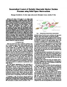
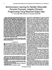
The approach here is similar to the previous case, i.e., R1 If λF ≤ ρ1 , then Vβ (p) = 1−β for all p ≤ ρ1 . If ρ1 < VI. N UMERICAL RESULTS −k λF ≤ ρ2 , let J +1 = min{k ∈ N : T (ρ1 ) < 0}. Let FJ+1 = We will first consider three different scenarios each one [0, T −J (ρ1 )] and Fi = (T −i (ρ1 ), T −(i−1) (ρ1 )] for 1 ≤ i ≤ J. of them leading to a different optimal policy. To validate the Then for p ∈ Fi , we have ρ2 > T i (p) > ρ1 ≥ T (i−1) (p), i.e., closed-form solutions obtained above we will also generate 1 − βi the optimal value function Vβ (p) using the value iteration Vβ (p) = R1 + β i Vβ,S (T i (p)). (22) algorithm. 1−β The parameters chosen below are selected in order to illustrate The optimal policy for this case is illustrated in Fig. 2. that in theory, any of the three policies could be optimal. The first set of parameters considered is λ0 = 0.2, λ1 = 0.9, τ = 0.4, R1 = 1, R2 = 2 and β = 0.1. Note that from a practical standpoint τ = 0.4 represents a substantial duration for sensing. As shown in Fig. 4, the optimal policy in this case is a Fig. 2. Illustration of the two thresholds policy for ρ1 < λF ≤ ρ2 . one threshold policy, whereas the two and three thresholds If λF > ρ2 , two cases can be distinguished; If T (ρ1 ) ≤ ρ2 policies are unfeasible in this case. If we keep all the parameter then the computation is similar to the situation where ρ1 < values fixed and diminish the sensing time to τ = 0.1, then λF ≤ ρ2 discussed above. If T (ρ1 ) > ρ2 , let FJ+1 = from Fig.5, we can see that the optimal policy becomes a [0, T −J (ρ1 )], for 2 ≤ i ≤ J let Fi = (T −i (ρ1 ), T −(i−1) (ρ1 )] two thresholds policy, whereas the one threshold policy gives and F1 = (T −1 (ρ1 ), T −1 (ρ2 )]. Then for p ∈ Fi , i ≥ 1, Vβ (p) suboptimal values (the three thresholds policy is unfeasible in this case). will be given by (22). For p ∈ F0 = (T −1 (ρ2 ), ρ1 ] we have Fig. 6 shows the optimal value function for the following Vβ (p) = R1 + βVβ,Th (T (p)). (23) settings: λ0 = 0.81, λ1 = 0.98, τ = 0.035, R1 = 2.91, R2 = 3 and β = 0.7. Here, the optimal policy is a three C. Three thresholds policy thresholds policy, and the one and two thresholds policies The goal is to find Vβ (p) for p ∈ [0, ρ1 ] ∪ [ρ2 , ρ3 ]. For provide suboptimal results. These numerical simulations prove p ∈ [ρ2 , ρ3 ], let J + 1 = min{k ∈ N : T −k (ρ3 ) < ρ2 }. Let that all scenarios can be possible and that our developed FJ+1 = [ρ2 , T −J (ρ3 )) and Fi = [T −i (ρ3 ), T −(i−1) (ρ3 )) for formulae give always the optimal policy. Finally, it should 1 ≤ i ≤ J. For p ∈ Fi , we have T i (p) ≥ ρ3 , i.e., Vβ (p) is be noted that finding a scenario where the optimal policy has given by (21). three-thresholds was not obvious. The parameters had to be For p ∈ [0, ρ1 ] we can distinguish two cases; repeatedly tuned in order to obtain such a case. If T (ρ1 ) ≤ ρ2 , Vβ (p) for p ∈ [0, ρ1 ] is computed using (22). Fig. 7 shows the effect of the sensing time τ on the length of If T (ρ1 ) > ρ2 , let H +1 = min{k ∈ N : T −k (ρ1 ) < 0}. Then the sensing region |ΦS | = ρ2 − ρ1 . The system parameters in we have two subcases: If T −(H+1) (ρ2 ) ≥ 0, then let ZH+1 = this plot are as follows: R1 = 1, R2 = 2, β = 0.99, λ0 = 0.1 [0, T −(H+1) (ρ2 )), for 1 ≤ i ≤ H let Zi = [T −i (ρ1 ), T −i (ρ2 )) and λ1 = 0.9. In this example, the two-thresholds policy is −i −(i−1) and for 1 ≤ i ≤ H + 1 let Qi = [T (ρ2 ), T (ρ1 )). optimal for τ ∈ [0, 0.537], and beyond this critical value,

9.88

2.4 Value iteration algorithm Proposed formulae

2.2

Proposed formulae (2 thresholds) Proposed formulae (1 threshold) Value iteration algorithm Proposed formulae (3 thresholds)

9.86 9.84 9.82

Vβ(p)

9.8

1.8 9.78

β

V (p)

2

1.6

9.76 9.74

1.4 9.72

0

1

0.1

0.2

0.3

0.4

0.5

0.6

0.7

0.8

0.9

1

p

1.2

Fig. 6. Optimality of a three thresholds policy. 0

0.2

0.4

0.6

0.8

1

1

p Fig. 4. Optimality of a one threshold policy.

0.9

R1=1, R2=2 β=0.99, λ =0.1, λ =0.9

0.8

0

1

0.7

2.4 ρ2 − ρ1

Value iteration algorithm Proposed formulae (2 thresholds) Proposed formulae (1 threshold)

2.2

0.6 0.5 0.4

2 1.8

0.2

β

V (p)

0.3

0.1

1.6

0

1.4

0

0.1

0.2

τ

0.3

0.4

0.5

Fig. 7. The effect of the sensing duration τ on ΦS .

1.2 1

0

0.2

0.4

0.6

0.8

1

p Fig. 5. Optimality of a two thresholds policy.

the one threshold policy will become optimal. As expected, the sensing region ΦS expands when the cost of sensing τ decreases until it covers the whole interval [0, 1] when τ = 0. VII. C ONCLUSION In this paper, we have studied a communication system operating over a Gilbert-Elliot channel. In order to maximize the number of successfully transmitted bits, the transmitter judiciously selects the best action among three possible options: i) transmit a high number of bits with no protection against a bad channel, ii) transmit a low number of bits but with perfect protection, iii) sense the channel for a fixed duration and then decide between the two previous actions. We have formulated the aforementioned problem as a Markov Decision Process, and we have established that the optimal strategy is a threshold policy. Namely, we have proved

that the optimal policy can have either one threshold, two thresholds, or three thresholds. We have provided closed-form expressions and simplified procedures for the computation of these policies as well as the resulting optimal number of transmitted bits. From a practical standpoint, the results presented in this paper could be used to optimize the channel utilization of real systems such as High-Speed Downlink Packet Access (HSDPA). A PPENDIX : C OMPUTATION OF Vβ (λ1 ) AND Vβ (λ0 ) Before giving the expressions of Vβ (λ1 ) and Vβ (λ0 ) we present an alternate expression for Vβ (p). This new expression will prove to be useful in the subsequent derivations. Theorem 3. The value function can be written as ½ ¾ 1 − βn n n n Vβ (p)=max R1+β max{Vβ,S (T (p)), Vβ,Th (T (p))} . n≥0 1 − β (25) Proof: See [12]. Intuitively the previous result can be explained as follows; The n n expression 1−β R + β Vβ,S (T n (p)) is the expected return 1 1−β when the transmitter selects n (≥ 0) times the action Tl , then selects the action S and the procedure continues on there on

optimality. Similarly for the other term but instead of taking the S action at the (n + 1)th stage, the action Th is selected. The value function is then just the maximum between these two expressions over all stages. Before proceeding with the computation of Vβ (λ1 ) and Vβ (λ0 ) we need the following lemma. Lemma 5. For the one and two-thresholds policies, let ΦTl = R1 [0, ρ). If λF ∈ ΦTl then Vβ (p) = 1−β for all p ∈ ΦTl . Proof: For all p ≤ λF , Vβ (p) = R1 + βVβ (T (p)), however, p ≤ T (p) ≤ λF , hence Vβ (T (p)) = R1 + βVβ (T 2 (p)), i.e., Vβ (p) = R1 (1 + β) + β 2 Vβ (T 2 (p)). By induction we obtain 1 − βn + β n Vβ (T n (p)) for all n. (26) Vβ (p) = R1 1−β We obtain the desired result by letting n → ∞ (since 0 ≤ β < 1). Similarly, for λF ≤ p ≤ ρ, Vβ (p) = R1 + βVβ (T (p)), however, p ≥ T (p) ≥ λF , hence by induction we arrive at the same conclusion. We are now ready to compute Vβ (λ1 ) and Vβ (λ0 ) for each policy individually. A. One threshold policy There are two possible scenarios: If λ1 ≤ ρ then since λF ≤ λ1 ≤ ρ, from lemma 5, we have R1 Vβ (λ1 ) = Vβ (λ0 ) = 1−β . If λ1 > ρ then Vβ (λ1 ) = Vβ,Th (λ1 ), i.e., Vβ (λ1 ) = λ1 R2 +β(1−λ1 )Vβ (λ0 ) and using (25), we have that Vβ (λ0 ) is 1−βλ1 a solution to the following equation ¾ ½ 1 − βn n n R1 + β Vβ,Th (T (λ0 )) Vβ (λ0 ) = max n≥0 1−β 1 − βn = max{ R1 + β n (κn R2 + β(Vβ (λ0 ) n≥0 1−β + κn (Vβ (λ1 ) − Vβ (λ0 ))))}, (27) where κn = T n (λ0 ) = (1 − αn+1 )λF . Hence solving for Vβ (λ0 ) we obtain ) ( 1−β n n 1−β R1 + β gn R2 Vβ (λ0 ) = max , (28) n≥0 1 − β n+1 [1 − (1 − β)gn ] κn where gn = 1−βλ . Note that the last maximization is just 1 a one dimensional search and is computationally inexpensive. Indeed, since 0 ≤ β < 1, the search for a maximum can be effectively restricted to values of n ≤ N , where N is a sufficiently large value such that β N ¿ 1. Once Vβ (λ0 ) and Vβ (λ1 ) have been computed for both cases, we retain the scenario that achieves the maximal values. Indeed, from (2), it is seen that the optimal policy is the one that gives the maximal value for any initial belief p. Hence, in particular, the threshold ρ should be tuned so as to maximize Vβ (λ0 ) and Vβ (λ1 ).

B. Two thresholds policy There are three possible scenarios: R1 If λ1 ≤ ρ1 then Vβ (λ1 ) = Vβ (λ0 ) = 1−β . If ρ1 ≤ λ1 ≤ ρ2 then Vβ (λ1 ) = Vβ,S (λ1 ), i.e., Vβ (λ1 ) =

(1−τ )[R1 +λ1 (R2 −R1 )]+β(1−λ1 )Vβ (λ0 ) . Hence, using (25) we 1−βλ1 n o 1−β n have Vβ (λ0 ) = maxn≥0 1−β R1 + β n Vβ,S (T n (λ0 )) .

Consequently, solving for Vβ (λ0 ) we obtain ( 1−β n ) R1 1−β +β n (1−τ )[(1−(1−β)gn )R1 +gn R2 ] Vβ (λ0 )=max . n≥0 1 − β n+1 [1 − (1 − β)gn ] (29) If λ1 ≥ ρ2 then Vβ (λ1 ) = Vβ,Th (λ1 ), i.e., Vβ (λ1 ) = λ1 R2 +β(1−λ1 )Vβ (λ0 ) . And, using (25), Vβ (λ0 ) is computed as 1−βλ1 follows Vβ (λ0 ) = max{X1 , X2 }, where X1 is given by (28) and X2 is given by ( 1−β n ) [ 1−β +β n (1−τ )(1−κn )]R1 +β n [gn − τ κn ]R2 X2=max . n≥0 1 − β n+1 [1 − (1 − β)gn ] (30) Again, once Vβ (λ0 ) and Vβ (λ1 ) have been computed for the three scenarios, we retain the scenario that gives the maximal values. C. Three thresholds policy Since λ1 ≥ λ1 R2 +β(1−λ1 )Vβ (λ0 ) 1−βλ1 max{X1,X2}, where

λF ≥ ρ3 , we have Vβ (λ1 ) = and Vβ (λ0 ) is calculated as Vβ (λ0 ) = X1 is given by (28) and X2 is given by

(30). ACKNOWLEDGEMENT The authors gratefully acknowledge the detailed comments and suggestions of Professor Qing Zhao (U.C. Davis). R EFERENCES [1] A. J. Goldsmith and S. Chua, “Variable-rate variable-power MQAM for fading channels,” IEEE Trans. Commun., vol. 45, pp. 1218-1230, Oct. 1997. [2] Q. Zhang and S. A. Kassam, “Finite-state Markov model for Rayleigh fading channels,” IEEE Trans. Commun., vol. 47, pp. 1688-1692, Nov. 1999. [3] E. N. Gilbert, “Capacity of a burst-noise channel,” Bell Syst. Tech. Jou., vol. 39, pp. 1253-1265, Sept. 1960. [4] L. Johnston and V. Krishnamurthy, “Opportunistic file transfer over a fading channel - A POMDP search theory formulation with optimal threshold policies,” IEEE Transactions Wireless Communications, vol. 5, no. 2, pp. 394-405, Feb. 2006. [5] D. Zhang and K. M. Wasserman, “Transmission schemes for time-varying wireless channels with partial state observations,” Proc. of INFOCOM, pp. 467-476, 2002. [6] Q. Zhao and B. M. Sadler, “A survey of dynamic spectrum access,” IEEE Signal Processing Magazine, vol. 55, no. 5, pp. 2294-2309, May, 2007. [7] S. M. Ross, “Quality control under Markovian deterioration,” Management Science vol. 17, no. 9, pp. 587-596, May 1971. [8] E. L. Sernik and S. I. Marcus, “On the computation of the optimal cost function for discrete time Markov models with partial observations,” Annals of Operations Research, vol. 29, pp. 471-512, Apr. 1991. [9] G. E. Monahan “Optimal stopping in a partially observable binaryvalued Markov chain with costly perfect information,” Journal of Applied Probability, vol. 19, pp.72-81, 1982. [10] R. Smallwood and E. Sondik, “The optimal control of partially observable Markov processes over a finite horizon,” Ops. Research, pp. 10711088, 1971. [11] S. M. Ross, “Applied probability models with optimization applications,” San Francisco: Holden-Day, 1970. [12] A. Laourine and L. Tong, “Betting on Gilbert-Elliot Channels,” Cornell University, Tech. Rep. ACSP TR-01-09-14, January 2009. [Online]. Available: http://acsp.ece.cornell.edu/papers/ACSP-TR-01-09-14.