482
IEEE TRANSACTIONS ON SYSTEMS, MAN, AND CYBERNETICS—PART B: CYBERNETICS, VOL. 31, NO. 4, AUGUST 2001
Neural Dynamic Optimization for Control Systems—Part I: Background Chang-Yun Seong, Member, IEEE, and Bernard Widrow, Life Fellow, IEEE
Abstract—The paper presents neural dynamic optimization (NDO) as a method of optimal feedback control for nonlinear multi-input-multi-output (MIMO) systems. The main feature of NDO is that it enables neural networks to approximate the optimal feedback solution whose existence dynamic programming (DP) justifies, thereby reducing the complexities of computation and storage problems of the classical methods such as DP. This paper mainly describes the background and motivations for the development of NDO, while the two other subsequent papers of this topic present the theory of NDO and demonstrate the method with several applications including control of autonomous vehicles and of a robot arm, respectively. Index Terms—Dynamic programming (DP), information time shift operator, learning operator, neural dynamic optimization (NDO), neural networks, nonlinear systems, optimal feedback control.
I. INTRODUCTION
N
ONLINEAR control system design has been dominated by linear control techniques, which rely on the key assumption of a small range of operation for the linear model to be valid. This tradition has produced many reliable and effective control systems [1]–[4]. However, the demand for control methods of complex nonlinear multi-input-multi-output (MIMO) systems has recently been increasing for several reasons. First, most real-world dynamical systems are inherently nonlinear. Second, modern technology, such as high-performance aircraft and high-speed high-accuracy robots, demands control systems with much more stringent design specifications, which are able to handle nonlinearities of the controlled systems more accurately. Third, along with the demand for high performance, MIMO control systems often become preferred or required because of the availability of cheaper and more reliable sensors and actuators made possible by the advances in such technology. The challenge for control design is to fully utilize this additional information and degrees of freedom to achieve the best control system performance possible. Fourth, controlled systems must Manuscript received January 16, 2000; revised February 11, 2001. This work was supported in part by the National Aeronautics and Space Administration under Contract NCC2-1020, the Office of Naval Research under Contract N00014-97-1-0947, and the National Science Foundation under Contract ECS–9522085. This paper was recommended by Associate Editor L. O. Hall. C.-Y. Seong was with the Information Systems Laboratory, Department of Electrical Engineering, Stanford University, Stanford, CA 94305 USA. He is now with Fineground Networks, Campbell, CA 95008 USA (e-mail:
[email protected]). B. Widrow is with the Information Systems Laboratory, Department of Electrical Engineering, Stanford University, Stanford, CA 94305 USA (e-mail:
[email protected]) Publisher Item Identifier S 1083-4419(01)05665-5.
be able to reject disturbances and uncertainties confronted in real-world applications. Unfortunately, there are few general practical feedback control methods for nonlinear MIMO systems [5], [6], although many methods exist for linear MIMO systems. The behavior of nonlinear systems is much more complicated and rich than that of linear systems because of both the lack of linearity and the associated superposition property [5], [7]. This paper presents neural dynamic optimization (NDO) as a practical method for nonlinear MIMO control systems. In order to handle the complexities of nonlinearity and accommodate the demand for high-performance MIMO control systems, NDO takes advantage of brain-like computational structures—neural networks—as well as optimal control theory. Our formulation allows neural networks to serve as nonlinear feedback controllers optimizing the performance of the resulting control systems. NDO is thus an offspring of both neural networks and optimal control theory. In optimal control theory [8]–[10], the optimal solution to a nonlinear MIMO control problem may be obtained from the Hamilton–Jacobi–Bellman equation (HJB) or the Euler–Lagrange (EL) equations . The two sets of equations provide the same solution in different forms: EL leads to a sequence of optimal control vectors, called feedforward optimal control (FOC); HJB yields a nonlinear optimal feedback controller, called dynamic programming (DP). DP produces an optimal solution that is able to reject disturbances and uncertainties as a result of feedback. Unfortunately, computation and storage requirements associated with DP solutions can be problematic, especially for high-order nonlinear systems, a problem known as the curse of dimensionality [8], [10], [11]. The linear quadratic regulator (LQR) derived from DP has thus been applied to designing controllers for nonlinear MIMO systems through the linearization of the systems around an equilibrium point [9], [10]. However, such linearization imposes limitations on the stability and performance of closed-loop systems since it causes a loss of information about large motions and is valid only near the equilibrium point. Neural networks [12]–[14], in contrast, have a massively parallel distributed structure, an ability to learn and generalize,1 and a built-in capability to adapt their synaptic weights to changes in the surrounding environments. Neural networks are inherently nonlinear—a very important property, particularly if the underlying physical mechanisms for the systems are highly nonlinear. More importantly, they can approximate any nonlinear function to a desirable accuracy [15]–[17]. 1Generalization refers to the neural network producing reasonable outputs for inputs not encountered during training (or learning).
1083–4419/01$10.00 ©2001 IEEE
SEONG AND WIDROW: NDO FOR CONTROL SYSTEMS—PART I: BACKGROUND
Thus, we propose an approximate technique for solving the DP problem based on neural network techniques that provides many of the performance benefits (e.g., optimality and feedback) of DP and benefits from the numerical properties of neural networks. We formulate neural networks to approximate optimal feedback solutions whose existence DP justifies. In other words, neural networks serve as building blocks for finding the optimal solution. As a result, NDO closely approximates—with a reasonable amount of computation and storage—optimal feedback solutions to nonlinear MIMO control problems that would be very difficult to implement in real-time with DP. Incidentally, the method developed in the paper is not the same as neurodynamic programming [18], which involves approximating the optimal solutions for discrete-state systems where the number of states is finite and the number of available controls at each state is also finite. However, the two methods are related since they try to achieve the same goal: approximating the optimal feedback solution using neural networks. The research presented in this paper was inspired by the works of Nguyen [19] and Plumer [20]. Nguyen showed the possibility of using neural networks in controlling a system with high nonlinearities by training them successfully to back up a trailer-truck to a loading dock. He primarily introduced a time-horizon-control concept to static neural network controllers, unraveling in time the feedback loop of the system-controller configuration to produce a large equivalent feedforward network. He applied the backpropagation algorithm [21], [22] to the large network to train the neural controller, which is called the backpropagation-through-time algorithm. He also pointed out the possibility of a connection between his work and optimal control theory. Plumer [20] extended Nguyen’s work; he explored a connection between the neural network control and optimal feedback control. He illustrated their connection by applying the static neural network controller to some nonlinear SISO systems in finite horizon problems, such as terminal control. However, static controllers may have limitations in finite horizon problems because the optimal feedback solutions to such problems are inherently time-varying [8], [9]. NDO can produce the time-varying as well as time-invariant optimal feedback solutions to nonlinear MIMO control problems. NDO can handle not only finite-horizon problems (e.g., terminal control) but also infinite-horizon problems (e.g., regulation and tracking control). NDO can produce the neural controllers that are able to minimize the effect of disturbances and uncertainties that may be confronted in real-world applications. This paper mainly describes the background and motivations for the development of NDO, while the two other subsequent papers [23], [24] of this topic present the theory of NDO and demonstrate the method with several applications including control of autonomous vehicles and of a robot arm, respectively. Four sections comprise this paper. Section II is an overview of optimal control theory, including DP, the LQR, and FOC. We point out the problematic aspects of optimal control theory, which in turn provide the motivation for this research. In any case, optimal control theory remains useful because it provides theoretical limits to the performance of NDO, the method presented in the paper. Section III reviews neural networks and their
483
Fig. 1. NTV-MIMO system.
properties, emphasizing their capability as general function approximators. Section IV provides conclusions. II. OPTIMAL CONTROL THEORY This section overviews optimal control theory, especially DP, the LQR, and FOC. A. Dynamic Programming (DP) DP finds optimal feedback solutions to nonlinear MIMO control problems. This approach fully exploits the state concept. Bellman derived the optimality condition for the optimal value of a cost function, and the control as a function of state using the principle of optimality [11], [25], [26]. A more descriptive name would be nonlinear optimal feedback control. Suppose we have a discrete nonlinear-time-varying (NTV) MIMO system described by a state equation of the form (1) is the state vector, and is the conwhere depends on the current trol input vector. The future state and the current input vector through a nonlinear state , which may have explicit time dependency. Fig. 1 function represents the NTV-MIMO system. A fairly general optimization approach finds the optimal feedback control to minimize a cost function of the form (2) subject to (1) with the time horizon and the function specpenalizes the state at the time ified. The function , and the function penalizes the states horizon and the control inputs through to . The and may have explicit time dependency, acfunctions cording to the goal of control. The optimal solution to the problem can be obtained by solving the discrete HJB equation. Theorem 1: For the given dynamic optimization problem of minimizing the cost function (3) subject to (4)
484
IEEE TRANSACTIONS ON SYSTEMS, MAN, AND CYBERNETICS—PART B: CYBERNETICS, VOL. 31, NO. 4, AUGUST 2001
where and the function are specified, the optimal feedback solutions are obtained from the discrete HJB equation (5) with the initial condition (6) Proof: The proof of the theorem is given in the literature [9], [11], [27]. First, HJB justifies the existence of a nonlinear optimal feedback solution. Second, in order to obtain the optimal solution, at the we need to find the optimal cost function2 at the time horizon as an initial condition. state Then, we solve HJB recursively backward in time over state space. However, HJB can be very difficult to solve for high-order nonlinear systems. To make the computational procedure feasible it is necessary to quantize the admissible state and control values into a finite number of levels. The computational procedure does not yield an analytical expression, but the optimal feedback control law is implemented by extracting the control values from a storage device that contains the solution of HJB in tabular form. To calculate the optimal control sequence for a given initial condition, we enter the storage location corresponding to the specified initial condition and extract the conand the minimum cost. Next, by solving the state trol value , which equation we determine the state of the system at at . The resulting value of results from applying is then used to reenter the table and extract , and so on. The optimal controller is physically realized by a table look-up device. In addition, storage requirements of the HJP solutions increase very rapidly with the state dimension. Bellman referred to this drawback as the curse of dimensionality. To appreciate the nature of the problem, we may consider a fourth-order SISO system with 0 quantization levels in each state coordinate as well as 0 time steps. The solution of HJB to the control problem restorage quires at least locations. Interpolation may also be required when one is using stored data to compute an optimal control sequence. For exdrives ample, if the optimal control applied at some value of that is halfway between two the system to a state value points where the optimal controls are 1 and 0, then by linear interpolation the optimal control is 0.5. Naturally, the degree of approximation depends on the separation of the grid points in state coordinates, the interpolation scheme used, the system dynamics, and the cost function. A finer grid generally means greater accuracy, but also means increased storage requirements and computation time. Linear Quadratic Problems: DP can be subject to intensive computation and extensive storage requirements, especially for high-order nonlinear systems. However, it produces important results for linear quadratic problems where systems are linear and cost functions are quadratic. 2The optimal cost function is also called the optimal return function or the optimal cost-to-go function.
Fig. 2. LTI-MIMO system.
Consider a discrete linear-time-invariant (LTI) MIMO system described by a state equation of the form (7) is the state vector and is the conwhere trol input vector. Fig. 2 depicts the discrete LTI-MIMO system. We want to find the optimal feedback control to minimize a constant-coefficient quadratic cost function
(8) , , and .3 with By applying the HJB (5) to the linear quadratic problem we may obtain the following result. Theorem 2: For the linear quadratic dynamic optimization problem of minimizing the cost function
(9) subject to (10) the optimal feedback controls are obtained from the following set of equations: (11) (12) (13)
(14) for (14) is given in (9). where the final condition Proof: The proof of the theorem is given in [9] and [10]. The HJB equation produces the set of solution equations for the linear quadratic problems. In order to obtain the optimal solution to the linear quadratic problems, we need to solve the Riccati (14) recursively backward in time. Then, we compute the 3If the system and weighting matrices vary according to time, the result to follow still holds.
SEONG AND WIDROW: NDO FOR CONTROL SYSTEMS—PART I: BACKGROUND
time-varying Kalman gain , using (12). The Riccati equation is much easier to solve than the HJB equation. We point out that the optimal feedback solution to the linear rather quadratic problem is a linear function of the state than a nonlinear one. In other words, DP shows that linear state feedback is the best form of feedback for linear quadratic problems. Thus the resulting closed-loop system is also linear like the open-loop system, which is an important result for linear control systems. Note also that optimal feedback controls for LTI systems with constant-coefficient quadratic cost functions has explicit are time-varying because the Kalman gain time-dependency. However, we may prefer a constant Kalman gain , which enables the closed-loop system to be LTI like the open-loop system. The next subsection will discuss the conditions under which we can obtain a constant Kalman gain for the linear quadratic problem.
485
The next theorem provides us with the conditions on the uniqueness of the bounded limiting solution as well as the asymptotical stability of the closed-loop system in terms of the observability of the system through the fictitious output. Theorem 4: Let be a square root of the intermediate-state , and suppose . weighting matrix, so that is observable. Then is controllable if Suppose and only if we have the following: 1) There is a unique positive definite limiting solution to the Riccati (14). Furthermore, is the unique positive definite solution to the ARE (16). 2) The closed-loop system
is asymptotically stable, where is given by (17). Proof: The proof of the theorem is given in [9] and [10].
B. Linear Quadratic Regulator (LQR) In Section II-A, where we considered the application of DP to linear quadratic problems, the closed-loop system is given by (15) The resulting closed-loop system is time-varying since the is time-varying even though the open-loop optimal gain system is time invariant. However, this time-varying feedback is not always convenient to implement: it requires the storage of an entire sequence matrices. Accordingly, we are interested in a constant of feedback gain. As one candidate for a constant feedback gain, as the time horizon we consider the limit of the optimal goes to infinity. We call this case the LQR [8]–[10]. does converge, then for a large If . Thus, in the limit, the Riccati (14) becomes the algebraic Riccati equation (ARE)
The controllability of , which is a dynamical property of the open-loop system, is crucial to guarantee that there exists a unique stabilizing optimal feedback solution to the linear quadratic regulation problem. We can pick without any difficulsuch that the observability of is ties a proper guaranteed. In other words, the open-loop system at least needs to be controllable to guarantee the unique optimal solution. We also point out that the ARE (16) is nonlinear with respect to unknown parameter . However, we can solve it easily using the DLQR command in MATLAB. The LQR has been applied to nonlinear MIMO feedback control design through linearization around an equilibrium point. However, such linearization may impose limitations on the stability and performance of closed-loop systems since it causes a loss of information about large motions and is valid only near the equilibrium point. C. Feedforward Optimal Control (FOC)
(16) which does not depend on time. The limiting solution to the Riccati (14) is clearly a solution of the ARE (16). The corresponding steady-state Kalman gain is (17) which is a constant feedback gain. The resulting closed-loop system is
FOC is an alternative method for nonlinear MIMO control problems. It treats the same dynamic optimization problem as DP and provides the same optimal solution in a different form: it finds the sequence of optimal control vectors with a specified initial state instead of the feedback solution for all possible initial states [8], [10]. It finds the optimal control solution relatively easily. However, its solution can be very sensitive to disturbances and uncertainties because of the lack of a feedback mechanism. Let us consider the same form of the discrete NTV-MIMO system as in the case of DP
(18) (19) which is also linear time invariant like the open-loop system. The following theorem tells us when there exists a bounded limiting solution . be controllable, then there is a Theorem 3: Let to (14). Furthermore, is a bounded limiting solution positive semidefinite solution to the ARE (16). Proof: The proof of the theorem is given in [9] and [10].
with (20) is the state vector and where control input vector. Note that an initial state and this was not done in the case of DP.
is the is specified here
486
IEEE TRANSACTIONS ON SYSTEMS, MAN, AND CYBERNETICS—PART B: CYBERNETICS, VOL. 31, NO. 4, AUGUST 2001
Here, we want to find the sequence of optimal control vectors for to minimize the same form of the cost function as in the case of DP. (21) , and the function specisubject to (19) and (20) with fied. Thus its optimal solution is not closed-loop but open-loop is no longer a function of the state . However, because this control problem is relatively easy to solve because it beas comes a parameter optimization problem by treating a set of unknown parameters. is obtained by The optimal control vector sequence solving the discrete EL equations. Theorem 5: For the given dynamic optimization problem of minimizing the cost function (22) subject to (23) with (24) , and the function are specified, the sequence where can be obtained from the of the optimal control vectors discrete EL equations. Proof: The proof of the theorem is given in [8]. Note that the EL equations consist of the system equation, the adjoint system equation, and the optimality condition: the system equation— (25) , with the adjoint system equation—
Fig. 3.
Forward sweep of FOC.
equations. It can be solved as a large set of simultaneous nonlinear algebraic equations (e.g., using the command FSOLVE in MATLAB). However, a more efficient method of solution, to be described in the next subsection, exploits the sequential nature of the problem. 1) Numerical Solution with Steepest Descent Method: We may apply steepest descent to obtain a numerical algorithm. The steepest descent algorithm for FOC, which exploits the sequential nature of EL, consists of three steps: 1) forward sweep; 2) backward sweep; 3) update of control vector sequence. Step 1) Forward sweep (31) . with The forward sweep equation is the same as the system equation. First of all, we need to make a reafrom through . sonable guess about Then with the specified initial state , we can comthrough to , using the system pute equation. Fig. 3 depicts the forward sweep. Step 2) Backward sweep (32)
(26) (33) with and the optimality condition—
(27) where we define (28) (29) (30) The system equation has an initial condition at the initial time , while the adjoint system equation has an initial condi. This is a two-point tion at the end of the time horizon and boundary value problem (TPBVP). Since both have dimension , has dimension , and , unknowns and an equal number of this TPBVP has
. with The backward sweep equations consist of the adjoint system equation and the optimality condition. These equations can be represented by a block diagram, as illustrated in Fig. 4. We have the , two co-inputs and co-state derived from the cost function, . and the co-output This system is anti-causal and linear-time-varying depends (LTV) because the current co-state through (32) on the future co-state and and the coefficients such as are explicitly time-dependent. and backHowever, we can compute ward in time because we have already obtained the and from the forward sweep. sequences of
SEONG AND WIDROW: NDO FOR CONTROL SYSTEMS—PART I: BACKGROUND
487
Fig. 5.
Fig. 4. Backward sweep of FOC.
Step 3) Update of control vector sequence (34) (35)
Forward sweep of FOC for linear quadratic problems.
a simpler form of the equations—an important structural property of computation, the so-called duality of the forward and the backward sweeps. By applying EL and the steepest descent method to the linear quadratic problem, we obtain the following three steps. Step 1) Forward sweep (38)
using (34) and (35). We reThen we update is small. peat the three steps until FOC is an alternative method for nonlinear MIMO control problems because it is relatively easy and computationally tractable to find its solution. The computation requirement of the FOC algorithm for each iteration is composed of three components: forward sweep, backward sweep, update of control vector sequence. The forward sweep multiplicarequires approximately tions and additions because it evaluates the system to . The backward sweep equation from operations needs roughly because it computes Jacobians and at each time step. The update of control vector sequence needs approximately operations. So the total number of multiplications and additions for each iteration using the FOC algorithm is approximately (36) The memory requirement of the algorithm is approximately (37) and the consince it needs to store the state from to . Note that the trol input memory requirement of FOC depends linearly on the dimension of the state and on the number of control inputs , while that of DP increases exponentially with and . However, FOC finds just a single trajectory for a given initial state. A severe problem for FOC is that its solutions are very sensitive to disturbances and uncertainties because of the lack of feedback. 2) Linear Quadratic Problems: The application of FOC to linear quadratic problems reveals—because FOC employs
. with The forward sweep equation is the same as the system equation. Fig. 5 depicts the forward sweep for linear quadratic problems. Step 2) Backward sweep (39) (40) . with The backward sweep equations consist of the adjoint system equation and the optimality condition as in the general case of FOC. These equations can be represented by the block diagram illustrated in , two co-inputs Fig. 6. We have the co-state and derived from the cost function, and . Comparing Fig. 5 with Fig. 6 the co-output reveals the duality of the backward and the forward sweeps. • The coefficient matrices of the backward sweep are the transpose of the coefficient of the forward sweep. matrices • The time advance operator in the backward sweep replaces the time delay operator in the forward sweep. • The directions of signal flows in the backward sweep are reversed to those in the feedforward sweep. • The summing junctions in the backward sweep replace the branching points in the forward sweep, and vice versa. Step 3 Update of control vector sequence: (41) (42) The update equations are the same as in the general case of FOC.
488
Fig. 6.
IEEE TRANSACTIONS ON SYSTEMS, MAN, AND CYBERNETICS—PART B: CYBERNETICS, VOL. 31, NO. 4, AUGUST 2001
Backward sweep of FOC for linear quadratic problems.
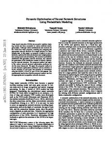
III. NEURAL NETWORKS This section reviews artificial neural networks, commonly referred to as neural networks. Neural networks are attractive in that they can approximate any nonlinear function to a desirable accuracy. In addition, neural networks possess other important properties. Neural networks have massively parallel distributed structures; implemented in hardware form, they can be inherently fault tolerant in the sense that their performance degrades gracefully under adverse operating conditions [28]. Neural networks can learn and generalize; generalization refers to the neural network producing reasonable interpolated outputs for inputs not encountered during learning (training) [29]. Neural networks are inherently nonlinear—a very important property, particularly if the underlying physical mechanism responsible for the generation of signals (e.g., a nonlinear MIMO system) is highly nonlinear. Neural networks have the built-in capability to adapt their synaptic weights to changes in the surrounding environment; a neural network trained to operate in a specific environment can be easily retrained to deal with minor changes in the operating environmental conditions [12]. An artificial neural network results from arranging a neuron model into various configurations. The most popular configuration is the multilayer feedforward network [12], [13], [29]. As illustrated in Fig. 7, it has layers of neurons, where the inputs to each neuron on a layer are identical, and equal to the collection of outputs from the previous layer (plus the augmented value “1”). The beginning layer of the network is called the input layer, its final layer is called the output layer, and all other layers of neurons are called the hidden layers. For multilayer neural . This means: networks, we use the following notation: The neural network has external inputs. There are neurons in the network’s first layer, neurons in the second layer, and so on. In addition, a single neuron extracted from the th layer of an -layer network is depicted in Fig. 7. The weight denotes and neuron in connections between neuron in layer are arranged in the form of the column layer . The weights . The weight vector is an vector such that -dimensional vector where is the total number of weights in the network. The output (activation value) of the -th neuron . Note that the th in layer is represented by the variable neuron in layer performs a weighted sum on its own input signals and passes the sum through an activation function ( ) to . The outputs in the final -th generate its own output layer corresponding to the overall outputs of the network. For
Fig. 7. Multilayer feedforward neural network consists of layers of neurons with each layer fully connected to the next layer. The network receives its q -dimensional input vector and generates its r -dimensional output vector. TABLE I MULTILAYER NEURAL NETWORK NOTATION
convenience we define a variable for the outputs. Thus . We also define as the external inputs to the network. The inputs may be viewed as a 0th layer that gives the relation This notation is summarized in Table I. Now define an input vector and output vector as follows (see Fig. 7):
Then,
the
feedforward network forms a mapping, , from the inputs of the input layer to the outputs of the final layer parameterized by the weight vector . Given the current model of the neuron, with fixed weights, this mapping is ; there are no internal dynamics or memory devices. Nevertheless, the following theorem makes the multilayer feedforward neural network a powerful tool for computation. Theorem 6: (General function approximators): and any function Given any , there exists a two-layer feedforward neural network that to within mean squared error accuracy. can approximate Proof: The proof of the theorem is given in [15]–[17]. functions are square-integrable functions over a bounded . The function space includes every function set that could ever arise in a practical problem. For example, it includes continuous functions and all discontinuous functions that are piecewise continuous on a finite number of subsets of a set . also includes more complicated functions that are only
SEONG AND WIDROW: NDO FOR CONTROL SYSTEMS—PART I: BACKGROUND
of mathematical interest. Thus, the neural network can approximate practically any nonlinear function to a desirable accuracy. Theoretically, two types of nonlinear activation function can be used: one is a signum (i.e., threshold) function and the other is a sigmoid function [12], [16], [22]. In practice, however, we desire activation functions that are sigmoidal. As a special case, linear neural networks—i.e., matrices that have linear activation functions—can approximate any linear function. However, this theorem does not explain how to find the weights of the neural network to approximate a nonlinear function to a desirable accuracy. IV. CONCLUSION As part of the background for the development of NDO, we overview optimal control theory, especially DP, the LQR, and FOC. We point out the problematic aspects as well as the performance benefits of each individual method. In particular, DP produces the optimal solution that is able to reject disturbances and uncertainties as a result of feedback. However, computation and storage requirement associated with DP solutions can be problematic, especially for high-order nonlinear systems. Thus, in the companion papers [23], [24], we propose NDO as an approximate technique for solving the DP problem based on neural network techniques that provides many of the performance benefits (e.g., optimality and feedback) of DP and benefits from the numerical properties of neural networks. Reference [23] presents the theory of NDO, and [24] demonstrates the method on several applications including control of autonomous vehicles and of a robot arm, respectively. REFERENCES [1] G. F. Franklin, J. D. Powell, and A. Emami-Naeini, Feedback Control of Dynamic Systems, Third ed. Reading, MA: Addison-Wesley, 1994. [2] G. F. Franklin, J. D. Powell, and M. L. Workman, Digital Control of Dynamic Systems, Third ed. Reading, MA: Addison-Wesley, 1998. [3] S. P. Boyd, Linear Controller Design: Limits of Performance. Englewood Cliffs, NJ: Prentice-Hall, 1991. [4] T. Kailath, Linear Systems. Englewood Cliffs, NJ: Prentice-Hall, 1980. [5] J. E. Slotine and W. Li, Applied Nonlinear Control. Englewood Cliffs, NJ: Prentice-Hall, 1991. [6] A. Isidori, Nonlinear Control Systems: An Introduction. New York: Springer-Verlag, 1989. [7] H. K. Khalil, Nonlinear Systems. New York: Macmillan, 1992. [8] A. E. Bryson, Dynamic Optimization. Menlo Park, CA: Addison-Wesley-Longman, 1999. [9] F. L. Lewis, Optimal Control, 2nd ed. New York: Wiley, 1995. [10] R. F. Stengel, Optimal Control and Estimation. New York: Dover, 1994. [11] R. E. Bellman, Dynamic Programming. Princeton, NJ: Princeton Univ. Press, 1957. [12] S. Haykin, Neural Networks: A Comprehensive Foundation, 2nd ed. Englewood Cliffs, NJ: Prentice-Hall, 1999. [13] B. Widrow and M. A. Lehr, “30 years of adaptive neural networks: Perceptron, Madaline, and backpropagation,” Proc. IEEE, vol. 78, pp. 1415–42, Sept. 1990. [14] R. Hecht-Nielsen, Neurocomputing. Reading, MA: Addison-Wesley, 1990. [15] A. N. Kolmogorov, “On the representation of continuous functions of many variables by superposition of continuous functions of one variable and addition,” Doklady Akademii Nauk SSR, vol. 114, pp. 953–56, 1957. [16] R. Hecht-Nielsen, “Kolmogorov’s mapping neural network existence theorem,” in Proc. IEEE 1st Int. Conf. Neural Networks, vol. III, San Diego, CA, 1987, pp. 11–4. [17] K. Hornik, “Multilayer feedforward networks are universal approximators,” Neural Netw., vol. 2, pp. 359–66, 1989.
489
[18] D. P. Bertsekas and J. N. Tsitsiklis, Neuro-Dynamic Programming. Belmont, MA: Athena Scientific, 1996. [19] D. Nguyen, “Applications of neural networks in adaptive control,” Ph.D. dissertation, Stanford Univ., Stanford, CA, 1991. [20] E. S. Plumer, “Optimal terminal control uising feedforward neural networks,” Ph.D. dissertation, Stanford Univ., Stanford, CA, 1993. [21] P. Werbos, “Beyond regression: New tools for prediction and analysis in the behavioral sciences,” Ph.D. dissertation, Harvard Univ., Cambridge, MA, 1974. [22] D. E. Rumelhart, G. E. Hinton, and R. J. Williams, “Learning internal representations by error propagation,” in Parallel Distributed Processing, D. E. Rumelhart and J. L. McClell, Eds. Cambridge, MA: MIT Press, 1986, vol. 1, ch. 8. [23] C. Seong and B. Widrow, “Neural dynamic optimization for control systems—Part II: Theory,” IEEE Trans. Syst., Man, Cybern. B, vol. 31, pp. 490–501, Aug. 2001. , “Neural dynamic optimization for control systems—Part III: Ap[24] plications,” IEEE Trans. Syst., Man, Cybern. B, vol. 31, pp. 502–513, Aug. 2001. [25] R. E. Bellman and S. E. Dreyfus, Applied Dynamic Programming. Princeton, NJ: Princeton Univ. Press, 1962. [26] R. E. Bellman and R. E. Kalaba, Dynamic Programming and Modern Control Theory. New York: Academic, 1965. [27] D. G. Luenberger, Introduction to Dynamic Systems: Theory, Models, & Applications. New York: Wiley, 1979. [28] G. R. Bolt, “Fault tolerance in artificial neural networks,” Ph.D. dissertation, York University, York, ON, Canada, 1992. [29] D. Rumelhart and J. McClell, Eds., Parallel Distributed Processing: Explorations in the Microstructure of Cognition. Cambridge, MA: MIT Press, 1986, vol. 1.
Chang-Yun Seong (M’01) received the B.S. and M.S. degrees in aerospace engineering from Seoul National University, Seoul, Korea, in 1990 and 1992, respectively, and the M.S. degree in electrical engineering and the Ph.D. degree in aeronautics and astronautics from Stanford University, Stanford, CA, in 1998 and 2000, respectively. He was a Research Engineer with the Systems Engineering Research Institute (SERI/KIST), Taejon, Korea, before he pursued his graduate studies at Stanford University. He is currently a Research Engineer with Fineground Networks, Campbell, CA. His research interests include neural networks, optimization, control systems, and digital signal processing. Dr. Seong is a member of AIAA. He was a recipient of the Outstanding Teaching Assistant Award from the AIAA Stanford Chapter in 1997.
Bernard Widrow (M’58–SM’75–F’76–LF’95) received the S.B., S.M., and Sc.D. degrees in electrical engineering from the Massachusetts Institute of Technology (MIT), Cambridge, in 1951, 1953, and 1956, respectively. He joined the MIT faculty and taught there from 1956 to 1959. In 1959, he joined the faculty of Stanford University, Stanford, CA, where he is currently Professor of Electrical Engineering. He is Associate Editor of several journals and is the author of about 100 technical papers and 15 patents. He is coauthor of Adaptive Signal Processing (Englewood Cliffs, NJ: Prentice-Hall, 1985) and Adaptive Inverse Control (Englewood Cliffs, NJ: Prentice-Hall, 1996). A new book, Quantization Noise, is in preparation. Dr. Widrow is a Fellow of AAAS. He received the IEEE Centennial Medal in 1984, the IEEE Alexander Graham Bell Medal in 1986, the IEEE Neural Networks Pioneer Medal in 1991, the IEEE Signal Processing Society Medal in 1998, the IEEE Millennium Medal in 2000, and the Benjamin Franklin Medal of the Franklin Institute in 2001. He was inducted into the National Academy of Engineering in 1995 and into the Silicon Valley Engineering Council Hall of Fame in 1999. He is a Past President and currently a Member of the Governing Board of the International Neural Network Society.