Neural Dynamics for Mobile Robot Adaptive Control - Semantic Scholar

Neural Dynamics for Mobile Robot Adaptive Control

Von der Fakultät Informatik, Elektrotechnik und Informationstechnik der Universität Stuttgart zur Erlangung der W¨ urde eines Doktors der Naturwissenschaften (Dr. rer. nat.) genehmigte Abhandlung

Vorgelegt von

Mohamed Oubbati aus Algerien

Hauptberichter: Prof. Dr. Paul Levi Mitberichter: Prof. Dr. Peter Göhner Tag der m¨ undlichen Pr¨ ufung: 27. Juni 2006

Institut f¨ ur Parallele und Verteilte Systeme der Universität Stuttgart 2006

Preface

This Thesis is submitted in partial fulfillment of the requirements for the degree of “Doktor der Naturwiessenschaften”(Dr. rer. nat.) at the Institute of Parallel and Distributed Systems of Stuttgart University. Prof. Dr. Paul Levi and Prof. Dr. Peter Göhner acted as referees. Summary of the Thesis In this thesis, we investigate how dynamics in recurrent neural networks can be used to solve some specific mobile robot problems. We have designed a motion control approach based on a novel recurrent neural network. The advantage of this approach is that, no knowledge about the dynamic model is required, and no synaptic weight changing is needed in presence of time varying parameters. Furthermore, this approach allows a single fixed-weight network to act as a dynamic controller for several distinct robots. To generate the robot behavior over time, we adopted the theory of neural fields. We designed a framework to navigate a robot to its goal in an unknown environment without any collisions with static or moving obstacles. In addition, we could optimize the target path through intermediate homebases. This framework has also produced a simple and elegant solution for the problem of moving multiple robots in formation. The objective was to acquire a target, avoid obstacles and keep a geometric configuration at the same time.

ii We have obtained successful results, both on simulations and on real experimentations. Index Terms: Autonomous mobile robots, recurrent neural networks, metalearning, adaptive control, adaptive identification, neural field, navigation, behaviorbased control, robot formation. Acknowledgment Over the last three years, I have had the privilege to meet many people who contributed either directly to my scientific work or to my quality of life in general. First of all, I would like to express my gratitude to my advisors Prof. Dr. Paul Levi and Dr. Michael Schanz for supporting me, and for giving me so much freedom to explore and discover solutions for robotics. Thanks go also to my colleagues of the RoboCup COPS-team, with whom I enjoyed to work. I would also like to acknowledge the many people in Marburg, Bonn, Bremen, and Stuttgart who have shown great kindness and support, both academically and administratively over the years. Many thanks to all my friends, who helped me in many ways. I am very grateful to the German Academic Exchange Service (DAAD) for funding my research. During four years, I have enjoyed my scholarship. . . Thanks a lot. Finally, I can find no words to express my sincere appreciation and gratitude to the German people for their hospitality, kindness, punctuality, and for their passion for science and work. Thank you Germany . . . Herzlichen Dank Deutschland. Mohamed Oubbati Stuttgart, June 2006

Zusammenfassung Zielsetzung Autonome mobile Systeme m¨ ussen in der Lage sein, sich in ihre Einsatzumgebung autonom zu bewegen und dabei zu wissen, auf welchen Wegen sie sicher an bestimmte Zielpunkte gelangen. Ziel dieser Arbeit ist die Entwicklung eines Ansatzes, der mittels recurrent neuronaler Netze genaue und sichere zielgerichtete Bewegungen ermöglicht und dabei die kinematischen und dynamischen Einschränkungen eines Roboters ber¨ ucksichtigt. Hierbei stellt sich die Frage, wie die Dynamik dieser Netze f¨ ur die Kontrolle des beobachtbaren Verhaltens des Roboters eingesetzt werden kann. Im Rahmen dieser Arbeit soll diese Frage theoretisch, numerisch sowie praktisch untersucht werden. Aufbau der Arbeit Die Popularität der neuronalen Netze liegt darin, dass sie eine sehr flexible Modellklasse beschreiben. Neuronale Netze, deren Konnektivitätsgraf keine geschlossenen Wege enthält, werden heute in vielen Anwendungen eingesetzt. Solche zyklenfreie (feedforward) Netze realisieren nichtlineare Abbildungen und sind mit einfachen Lernverfahren trainierbar, besitzen jedoch keine eigene Dynamik. Rekurrente Netze, die durch einen Konnektivitätsgraf mit geschlossenen Wegen gekennzeichnet sind, besitzen dagegen ein weit reichenderes Spektrum an Verhaltensmöglichkeiten, da sie eine echte Dynamik aufweisen. Sie sind jedoch in ihrem Verhalten schwerer zu beherrschen und wurden daher in Anwendungen bisher selten eingesetzt. Als Grundlage der Arbeit, wird zu Beginn ein Konstruktives Lernverfahren f¨ ur rekurrente neuronale Netze untersucht, welches nur die Ausgabeneuronen f¨ uhrenden Verbindungen modifiziert, um das Lernziel zu erreichen. Diese Untersuchung ist durch einen speziellen Typ eines rekurrenten Netzes motiviert (Echo State Network, ESN), das in dieser Arbeit vor allem

iv aus Interesse an seiner Fähigkeit einfacher Lernverfahren, näher untersucht und f¨ ur die Robotiksteuerung angepasst. Zudem wird gezeigt, dass das ESN ¨ durch metalearning ohne Anderungen seiner Parameter ein adaptives Verhalten hat. Darauf aufbauend wird zunächst das ESN zur Identifikation nichtlinearer dynamischer Systeme behandelt. Hierf¨ ur werden nichtlineare dynamische Systeme ausgewählt, die durch nichtlineare Differenzengleichungen mit zeitvarianten Faktoren beschrieben werden. Es wird gezeigt, dass das ESN im Zusammenhang mit metalearning sehr gute Identifikationsergebnisse liefert und eine effektivere adaptive Echtzeitidentifikation im Vergleich zu anderen bekannten Verfahren ermöglicht. Zur Steuerung autonomer mobiler Roboter wird anhand des Robotersmodells eine adaptive Geschwindigkeitsregelung mittels eines ESN entworfen, simuliert, realisiert und auf einem realen Roboter getestet. In der Simulation wird ein Neurokontrol-System mit zwei Ebenen entwickelt. Die eine Ebene (dynamic-level) f¨ ur die adaptive Kontrolle des dynamischen Modells, die auf dem ESN und metalearning basiert; die zweite Ebene (kinematiclevel) f¨ ur das kinematische Modell, die auf einem anderen ESN basiert. Um die Robustheit zu verbessern, wurde während des Trainings zusätzlich ein Geräusch hinzugefgt. Hierbei konnten positive Ergebnisse erzielt werden. Auf dem realen Roboter wird ein ESN zu einem Pulsweitenmodulationsregler ausgebildet, der aufgrund der gegebenen aktuellen Geschwindigkeiten und der Sollgeschwindigkeiten die korrekten Parameter der Pulsweitenmodulation bestimmt. Ein Vorteil dieses Ansatzes ist die Anpassung der Radgeschwindigkeitsreglung ohne dass vorher Kenntnisse u ¨ber die dynamischen Eigenschaften des Roboters vorliegen m¨ ussen. Zudem kann sich ein einmal vortrainierter ESN-Regler bei Variation der Roboterphysik, z.B. bei Gewichtsveränderungen, ¨ ¨ ohne Anderungen seiner Parameter, auf die Anderungen relativ schnell einstellen. Diese Methode ermöglicht auch die gleichzeitige Geschwindigkeitsregelung drei unterschiedlicher Roboter mit einem einzigen vortrainierten ESN-Regler. Zur Navigation werden dynamische Systeme verwendet, um Navigationsverhalten f¨ ur einen oder mehrere autonome Roboter zu produzieren. Insbesondere soll ein biologisch motiviertes neuronales Feldmodell genutzt werden, um ein stabiles Verhalten eines Roboters zu erzeugen. Neuronale Felder sind skalare räumlich kontinuierliche Aktivitätsverteilungen, die typischerweise die Aktivität des Neokortex beschreiben. Die Felddynamik ist durch

v nichtlineare Integral-Differentialgleichungen beschrieben, die sich folgendermaßen darstellen: Der Ort der Neuronen wird durch die kontinuierliche Variable x bezeichnet. Eine orts- und zeitabhängige Funktion (Aktivierung) u(x, t) repräsentiert dann den Zustand der Dynamik an jedem Ort x zur Zeit t. Unter Annahme der Gleichgewichtslösung und externer Stimuli wird ein einziger Gipfel, im Folgenden “Peak” genannt, auf dem Feld erzeugt. In diesem Fall werden die Verhalten Hindernisvermeidung und Zielanfahrt durch das Feldmodell generiert. Zuerst werden alle möglichen Richtungseinstellungen des Roboters kodiert; dann gibt der Ort, an dem ein Peak generiert wurde, die Soll-Vorausrichtungen an. Eine vorgeschlagene Richtung wird ¨ solange beibehalten bis eine Anderung in der Umwelt auftritt. Hierdurch wird gezeigt, dass die stabilen Entscheidungen der neuronalen Felder, eine sichere Bewegung unter Vermeidung von statischen und dynamischen Hindernissen ermöglichen. Neben der Möglichkeit, Hindernisse zu vermeiden, wird das entwickelte lokale Navigationsystem angepasst, um auf dem Weg zum Zielpunkt zusätzlich homebases anzusteuern. Dar¨ uberhinaus wird im Rahmen dieser Arbeit ein Navigationsystem zur koordinierten Steuerung eines Multirobotersystem entwickelt. Es wird eine Neuronale Felder Strategie vorgestellt, mit der es möglich ist, eine Gruppe von Robotern zu steuern, die ihren Zielpunkt erreichen, eine Formation beibehalten, und Kollisionen mit Hindernissen oder miteinander vermeiden. Schlagw¨ orter: Mobile Roboter, Autonome Navigation, Rekurrente Neuronale Netze, Adaptive Regelung, Adaptive Identifikation, Metalearning, Verhaltensbasierte Kontrolle, Neuronale Felder.

Contents 1 Introduction 1.1 What sort of thesis is this? . . . . . . . 1.1.1 Tasks . . . . . . . . . . . . . . 1.1.2 How these tasks are addressed? 1.2 Issues and Goals . . . . . . . . . . . . 1.2.1 Motion Control . . . . . . . . . 1.2.2 Behavior Generation . . . . . . 1.3 Contributions . . . . . . . . . . . . . . 1.4 Outline of the Thesis . . . . . . . . . .

. . . . . . . .

. . . . . . . .

. . . . . . . .

. . . . . . . .

. . . . . . . .

. . . . . . . .

. . . . . . . .

. . . . . . . .

. . . . . . . .

2 Related Work 2.1 Control Architectures . . . . . . . . . . . . . . . . . . . 2.1.1 Deliberative Control . . . . . . . . . . . . . . . 2.1.2 Reactive Control . . . . . . . . . . . . . . . . . 2.1.3 Hybrid Control . . . . . . . . . . . . . . . . . . 2.2 Behavior-based Control . . . . . . . . . . . . . . . . . . 2.2.1 Behavior Coordination . . . . . . . . . . . . . . 2.2.2 Arbitration Mechanisms . . . . . . . . . . . . . 2.2.3 Fusion Mechanisms . . . . . . . . . . . . . . . . 2.3 Dynamical Systems Approach . . . . . . . . . . . . . . 2.3.1 Behavioral Variables . . . . . . . . . . . . . . . 2.3.2 Behavioral dynamics . . . . . . . . . . . . . . . 2.3.3 Dynamical systems for mobile robot navigation 2.4 Motion Control . . . . . . . . . . . . . . . . . . . . . . 2.4.1 Background . . . . . . . . . . . . . . . . . . . . 2.4.2 Motion Control with Neural Networks . . . . .

. . . . . . . . . . . . . . . . . . . . . . .

. . . . . . . . . . . . . . . . . . . . . . .

. . . . . . . . . . . . . . . . . . . . . . .

. . . . . . . .

2 2 2 2 3 3 4 4 7

. . . . . . . . . . . . . . .

10 10 10 11 11 12 13 13 14 14 14 15 15 19 19 21

CONTENTS

vii

3 Recurrent Neural Networks 3.1 Introduction . . . . . . . . . . . . . . . . . . . . . . . . . . . . 3.2 Artificial Neural Networks . . . . . . . . . . . . . . . . . . . . 3.2.1 Training of ANNs . . . . . . . . . . . . . . . . . . . . . 3.2.2 Neural Networks Topologies . . . . . . . . . . . . . . . 3.3 Learning in Recurrent Neural Networks . . . . . . . . . . . . . 3.3.1 Backpropagation Through Time . . . . . . . . . . . . . 3.3.2 Real-Time Recurrent Learning . . . . . . . . . . . . . . 3.3.3 Difficulty of learning long-term dependencies. . . . . . 3.3.4 Long Short-Term Memory . . . . . . . . . . . . . . . . 3.3.5 Extended Kalman Filter for RNNs Weight Estimation . 3.3.6 Temporal Integration in RNNs . . . . . . . . . . . . . . 3.3.7 Liquid State Machine . . . . . . . . . . . . . . . . . . . 3.4 Echo State Network . . . . . . . . . . . . . . . . . . . . . . . . 3.4.1 Formal Description . . . . . . . . . . . . . . . . . . . . 3.4.2 How ESN approach works? . . . . . . . . . . . . . . . . 3.4.3 Training Algorithm . . . . . . . . . . . . . . . . . . . . 3.5 Conclusion . . . . . . . . . . . . . . . . . . . . . . . . . . . . .

22 22 23 24 24 25 26 28 30 30 31 32 33 35 35 36 38 40

4 Metalearning 4.1 Review of Metalearning . . . . . . . . . . . . . . . . . . 4.1.1 Inductive Transfert . . . . . . . . . . . . . . . . 4.1.2 Dynamic Selection of Bias . . . . . . . . . . . . 4.1.3 Meta-learner of Base-learners . . . . . . . . . . 4.1.4 Lifelong Learning . . . . . . . . . . . . . . . . . 4.1.5 Multitask Learning . . . . . . . . . . . . . . . . 4.2 Fixed-Weight Neural Networks . . . . . . . . . . . . . . 4.2.1 Learning Learning Rules . . . . . . . . . . . . . 4.2.2 Multiple Modeling . . . . . . . . . . . . . . . . 4.3 Adaptive Identification with Fixed-Weight ESN . . . . 4.3.1 Preliminaries on Nonlinear System Identification 4.3.2 Problem Statement . . . . . . . . . . . . . . . . 4.3.3 Procedure . . . . . . . . . . . . . . . . . . . . . 4.3.4 Results . . . . . . . . . . . . . . . . . . . . . . . 4.4 Conclusion . . . . . . . . . . . . . . . . . . . . . . . . .

42 43 44 44 45 46 47 47 48 50 52 52 53 53 54 61

. . . . . . . . . . . . . . .

. . . . . . . . . . . . . . .

. . . . . . . . . . . . . . .

. . . . . . . . . . . . . . .

CONTENTS

viii

5 Control of Nonholonomic Robots with ESNs 5.1 Introduction . . . . . . . . . . . . . . . . . . . . . . . 5.2 Nonholonomic Mobile Robots . . . . . . . . . . . . . 5.2.1 Kinematic and Dynamic Modeling . . . . . . . 5.3 Motion control . . . . . . . . . . . . . . . . . . . . . 5.4 Dynamic-level Control with ESNs . . . . . . . . . . . 5.4.1 Procedure . . . . . . . . . . . . . . . . . . . . 5.4.2 Results . . . . . . . . . . . . . . . . . . . . . . 5.5 Adaptive Dynamic Control using Fixed-Weight ESNs 5.5.1 Problem Statement . . . . . . . . . . . . . . . 5.5.2 Procedure . . . . . . . . . . . . . . . . . . . . 5.5.3 Results . . . . . . . . . . . . . . . . . . . . . . 5.6 Control of Multiple Distinct Robots . . . . . . . . . . 5.6.1 Procedure . . . . . . . . . . . . . . . . . . . . 5.6.2 Results . . . . . . . . . . . . . . . . . . . . . . 5.7 Kinematic and Dynamic Adaptive Control with ESNs 5.7.1 ESN Kinematic Controller . . . . . . . . . . . 5.7.2 ESN Dynamic Adaptive Controller . . . . . . 5.7.3 Kinematic-Dynamic closed loop control . . . . 5.7.4 Results . . . . . . . . . . . . . . . . . . . . . . 5.8 Discussion . . . . . . . . . . . . . . . . . . . . . . . . 5.9 Conclusion . . . . . . . . . . . . . . . . . . . . . . . . 6 Control of an Omnidirectional Robot with 6.1 Introduction . . . . . . . . . . . . . . . . . 6.2 Omnidirectional Robot . . . . . . . . . . . 6.2.1 Hardware . . . . . . . . . . . . . . 6.2.2 Kinematic Model . . . . . . . . . . 6.2.3 Control System . . . . . . . . . . . 6.2.4 Problem Statement . . . . . . . . . 6.3 Velocity Control with ESN . . . . . . . . 6.3.1 Training . . . . . . . . . . . . . . . 6.3.2 Control Procedure . . . . . . . . . 6.3.3 Results . . . . . . . . . . . . . . . . 6.4 Fixed-Weight ESN Adaptive Controller . . 6.4.1 Procedure . . . . . . . . . . . . . . 6.4.2 Results . . . . . . . . . . . . . . . . 6.5 Discussion . . . . . . . . . . . . . . . . . .

ESNs . . . . . . . . . . . . . . . . . . . . . . . . . . . . . . . . . . . . . . . . . . . . . . . . . . . . . . . .

. . . . . . . . . . . . . .

. . . . . . . . . . . . . .

. . . . . . . . . . . . . . . . . . . . . . . . . . . . . . . . . . .

. . . . . . . . . . . . . . . . . . . . . . . . . . . . . . . . . . .

. . . . . . . . . . . . . . . . . . . . . . . . . . . . . . . . . . .

. . . . . . . . . . . . . . . . . . . . . . . . . . . . . . . . . . .

. . . . . . . . . . . . . . . . . . . . .

63 63 64 65 69 71 71 72 75 75 75 76 78 78 79 82 82 84 84 86 89 90

. . . . . . . . . . . . . .

92 93 93 94 95 97 97 98 98 98 99 103 103 104 108

CONTENTS 6.6

ix

Conclusion . . . . . . . . . . . . . . . . . . . . . . . . . . . . . 108

7 Neural Fields for Behavior Generation 7.1 Introduction . . . . . . . . . . . . . . . . . . . . . . . . 7.2 Neural Fields . . . . . . . . . . . . . . . . . . . . . . . 7.3 Dynamical Properties of Neural Fields . . . . . . . . . 7.3.1 Equilibrium Solutions in the Absence of Inputs 7.3.2 Response to Stationary Input Stimulus . . . . . 7.4 Behavior control with neural fields . . . . . . . . . . . 7.4.1 Control Design . . . . . . . . . . . . . . . . . . 7.4.2 Results . . . . . . . . . . . . . . . . . . . . . . . 7.5 Competitive Dynamics for Home-bases Acquisition . . 7.5.1 Sub-target Neural Field . . . . . . . . . . . . . 7.5.2 Target-acquisition Stimulus . . . . . . . . . . . 7.5.3 Results . . . . . . . . . . . . . . . . . . . . . . . 7.6 Neural Fields for Multiple Robots Control . . . . . . . 7.6.1 Control Design . . . . . . . . . . . . . . . . . . 7.6.2 Field Stimulus . . . . . . . . . . . . . . . . . . . 7.6.3 Formation Control . . . . . . . . . . . . . . . . 7.7 Results . . . . . . . . . . . . . . . . . . . . . . . . . . . 7.8 Conclusion . . . . . . . . . . . . . . . . . . . . . . . . .

. . . . . . . . . . . . . . . . . .

. . . . . . . . . . . . . . . . . .

. . . . . . . . . . . . . . . . . .

110 . 110 . 111 . 113 . 113 . 114 . 115 . 115 . 118 . 126 . 127 . 128 . 129 . 132 . 133 . 134 . 135 . 138 . 147

8 Neural Fields for Behavior-Based Control of a RoboCup Player148 8.1 Robot System . . . . . . . . . . . . . . . . . . . . . . . . . . . 149 8.1.1 Environment Sensing . . . . . . . . . . . . . . . . . . . 149 8.1.2 Self-Localization . . . . . . . . . . . . . . . . . . . . . 150 8.1.3 Software Architecture . . . . . . . . . . . . . . . . . . . 150 8.2 Neural Fields . . . . . . . . . . . . . . . . . . . . . . . . . . . 151 8.2.1 Equilibrium Solutions . . . . . . . . . . . . . . . . . . . 152 8.3 Control Design . . . . . . . . . . . . . . . . . . . . . . . . . . 153 8.3.1 Field Stimulus . . . . . . . . . . . . . . . . . . . . . . . 153 8.3.2 Dynamics of Speed . . . . . . . . . . . . . . . . . . . . 154 8.4 Results . . . . . . . . . . . . . . . . . . . . . . . . . . . . . . . 155 8.5 Conclusion . . . . . . . . . . . . . . . . . . . . . . . . . . . . . 161 9 Conclusions and future work 162 9.1 Summary of Contributions . . . . . . . . . . . . . . . . . . . . 162 9.2 Conclusions . . . . . . . . . . . . . . . . . . . . . . . . . . . . 163

CONTENTS 9.3

x

Future Directions . . . . . . . . . . . . . . . . . . . . . . . . . 164

List of Figures 2.1 2.2 2.3

SPA Architecture. . . . . . . . . . . . . . . . . . . . . . . . . Behavior-based Control . . . . . . . . . . . . . . . . . . . . . The dynamics of heading direction ϕ for target-acquisition. An attractor is generated at the direction ϕtar . . . . . . . . . . . 2.4 The dynamics of heading direction ϕ for obstacle-avoidance. A repellor is generated at the direction ϕobs . . . . . . . . . . 2.5 Attractor and Repellor interaction . . . . . . . . . . . . . . . 3.1 Artificial Neural Networks. a) Feedforward Neural Network. b) Partially connected RNN. c) Full connected RNN. . . . . 3.2 Backpropagation Through Time. a) recurrent neural network. b) network unfolded in time. . . . . . . . . . . . . . . . . . . 3.3 Left: A fully recurrent hidden network. Right: LSTM network with a memory bloc. . . . . . . . . . . . . . . . . . . . . . . 3.4 Basic architecture of Liquid State Machine. . . . . . . . . . . 3.5 Basic architecture of ESN. Dotted arrows indicate connections that are possible but not required. . . . . . . . . . . . . . . 4.1 4.2 4.3 4.4 4.5 4.6

Base-level learning . . . . . . . . . . . . . . . . . . . . . . . Meta-learning . . . . . . . . . . . . . . . . . . . . . . . . . . Multitask Learning of L tasks with the same inputs. . . . . A weight adaptation of a single unit network. . . . . . . . . A fixed-weight network equivalent to a single unit network. . Results of example 1. (a). Teacher output. (b). ESN Prediction test on new I/O data. Desired (solid) and network prediction (dashed) signals. . . . . . . . . . . . . . . . . . .

. 11 . 13 . 17 . 18 . 19 . 25 . 27 . 31 . 34 . 36 . . . . .

44 46 47 49 49

. 56

LIST OF FIGURES 4.7

4.8

5.1 5.2 5.3 5.4 5.5 5.6 5.7 5.8

5.9

5.10

5.11

5.12 5.13

5.14 5.15

xii

Results of example 2 (1st test). (a). Teacher output. (b). ESN Prediction test on new I/O data. Desired (solid) and network prediction (dashed) signals. . . . . . . . . . . . . . . . 59 Results of example 2 (2nd test). System(solid) vs ESN Prediction(dashed). (a). Responses to u1 (k). (b). Responses to u2 (k). . . . . . . . . . . . . . . . . . . . . . . . . . . . . . . . 60 Mobile robot with two actuated wheels. . . . . . . . . . . . . . Motion control using the kinematic model. . . . . . . . . . . . Two-stage model of a real mobile robot. . . . . . . . . . . . . Inner loop control of a mobile robot (dynamic-level control). . Control of a real mobile robot. . . . . . . . . . . . . . . . . . . Training ESND as a dynamic controller. . . . . . . . . . . . . Exploitation of ESND as a dynamic controller. . . . . . . . . . ESN adaptive velocity tracking control. a) Linear velocity tracking. b) Angular velocity tracking. c) Computed torque for wheel right. d) Computed torque for wheel left. . . . . . . ESN adaptive velocity tracking control. a) Linear velocity tracking. b) Angular velocity tracking. c) Computed torque for wheel right. d) Computed torque for wheel left. . . . . . . Linear and Angular velocity tracking (left) and controls (right). Each robot is controlled separately with the same fixed-weight ESN controller. . . . . . . . . . . . . . . . . . . . . . . . . . . Linear and Angular velocity tracking (left) and controls (right). The fixed-weight ESN controls the three robots, following swithes between them. The first switch occurs at time 25s from Robot II to I. The second switch occurs at time 35s from Robot I to III. . . . . . . . . . . . . . . . . . . . . . . . . . . . . . . . . . Training ESNK as a kinematic controller. . . . . . . . . . . . . Kinematic control. a) Robot trajectory tracking controlled by the two controllers separately. b)Tracking errors resulted from the feedback controller (K1 = K2 = K3 = 5). c) Tracking errors resulted from the ESNK control. . . . . . . . . . . . . . Global control structure of a nonholonomic mobile robot using ESNs . . . . . . . . . . . . . . . . . . . . . . . . . . . . . . . . Kinematic and dynamic control. a) Linear velocity tracking. b) Angular velocity tracking. c) Computed torque for wheel right. d) Computed torque for wheel left. e)Trajectory Tracking

66 69 69 70 70 72 72

74

77

80

81 83

85 86

88

LIST OF FIGURES 6.1 6.2 6.3 6.4 6.5 6.6 6.7

Omnidirectional robot. a)hardware photo. b) CAD model . An image from the omnidirectional camera. . . . . . . . . . Kinematic geometry of the Omnidirectional Robot. . . . . . Kinematic and dynamic control loops. . . . . . . . . . . . . Structure of the control system. . . . . . . . . . . . . . . . Structure of the control system. . . . . . . . . . . . . . . . Results of Experiment 1. Desired velocity(solid) and actual robot velocity (dashed). . . . . . . . . . . . . . . . . . . . . 6.8 Results of Experiment 2. Desired velocity(solid) and actual robot velocity (dashed). . . . . . . . . . . . . . . . . . . . . 6.9 Control results of the case 1. a) Desired speeds(solid), Wheels speeds (initial mass)(dashed), and Wheels speeds (mass=17.5 Kg) (dash dot). b) ESN control signals initial mass)(dashed). ESN control signals (mass=17.5 Kg) (dash dot) . . . . . . . 6.10 Control results of the case 2. a) Desired speeds(solid) and actual Wheels speeds (dashed), b) ESN control signals . . . 7.1 7.2 7.3 7.4 7.5 7.6 7.7 7.8 7.9 7.10 7.11 7.12 7.13 7.14 7.15 7.16

Weihting function w(x) of a lateral-inhibition . . . . . . . . Target acquisition with Obstacle avoidance . . . . . . . . . . Collision Avoidance for Moving Obstacles. The dotted lines in (e) represent the old positions of the obstacles. . . . . . . Corridor Following: experiment 1 . . . . . . . . . . . . . . . Corridor Following: experiment 2 . . . . . . . . . . . . . . . Door Passing . . . . . . . . . . . . . . . . . . . . . . . . . . Sub-targets Acquisition . . . . . . . . . . . . . . . . . . . . . Sub-target Acquisition Through Competition . . . . . . . . . Sub-targets Acquisition: Flexibility . . . . . . . . . . . . . . Geometric Configurations: a) line, b) column, c) triangle . . Triangle and Line Configuration . . . . . . . . . . . . . . . . Column Configuration . . . . . . . . . . . . . . . . . . . . . Line configuration in obstacle free situation. a)Robots’ headings. b) Robots’ velocities . . . . . . . . . . . . . . . . . . . Line configuration with obstacles. a)Robots’ headings. b) Robots’ velocities . . . . . . . . . . . . . . . . . . . . . . . . Line configuration with moving target and fixed obstacles. a)Robots’ headings. b) Robots’ velocities . . . . . . . . . . . Triangle configuration. a)Robots’ headings. b) Robots’ velocities . . . . . . . . . . . . . . . . . . . . . . . . . . . . . . .

xiii . . . . . .

92 95 96 97 99 99

. 101 . 102

. 105 . 107 . 113 . 120 . . . . . . . . . .

121 123 124 125 127 130 131 133 137 137

. 139 . 140 . 141 . 142

LIST OF FIGURES 7.17 Triangle configuration with moving target. a)Robots’ headings. b) Robots’ velocities . . . . . . . . . . . . . . . . . . . 7.18 Triangle configuration with moving target and fixed obstacles. a)Robots’ headings. b) Robots’ velocities . . . . . . . . . . . 7.19 Column configuration in a door passing test. a)Robots’ headings. b) Robots’ velocities . . . . . . . . . . . . . . . . . . . 7.20 Column configuration in a door passing test. a)Robots’ headings. b) Robots’ velocities . . . . . . . . . . . . . . . . . . . 8.1 8.2

8.3 8.4 8.5 8.6 8.7 8.8

xiv

. 143 . 144 . 145 . 146

Omnidirectional robot. a)hardware photo. b) CAD model . . 148 Information extraction from the camera a) Image captured from the omni-camera b) Recognition of relevant objects: lines(white), ball(red), obstacles (black), and goals (blue and yellow). . . . 150 Robot Software Architecture. . . . . . . . . . . . . . . . . . . 151 Target acquisition with Obstacle avoidance: first experiment . 157 Target acquisition with Obstacle avoidance: second experiment 158 Photos from video sequences of the first experience. . . . . . . 159 Photos from video sequences of the second experience. . . . . 159 Target acquisition with moving obstacle avoidance . . . . . . . 160

List of Tables 4.1

System parameters values and their time intervals . . . . . . . 58

5.1 Values of mc and d in their time intervals . . . . . . . . . . . . 77 5.2 Robots Specifications . . . . . . . . . . . . . . . . . . . . . . . 78 5.3 . . . . . . . . . . . . . . . . . . . . . . . . . . . . . . . . . . . 87 6.1 Robot Specifications . . . . . . . . . . . . . . . . . . . . . . . 95

Chapter 1 Introduction

1.1

What sort of thesis is this?

This thesis is a robotics thesis. We address issues of machine learning. We investigate how recurrent neural networks can offer efficient and practical solutions. We design adaptive systems. But, this thesis describes progress towards the ultimate goal of mobile robotics: “move a robot safely and precisely in real environments”.

1.1.1

Tasks

Two main tasks are addressed in this work. The first task is designing an adaptive motion control system. The second is the behavior-based control of single and multiple mobile robots. Both of these tasks involve real-world constraints.

1.1.2

How these tasks are addressed?

The primary methods we used for solving our robotics problems are based on recurrent neural network (RNN) techniques. The ability of RNNs to instantiate arbitrary temporal dynamics allows us to design motion control, includ-

1.2 Issues and Goals

3

ing also the dynamics part of the robot. Moreover, through metalearning, no synaptic weight changing is needed in presence of parameters variation. The concept of dynamic stability in neural fields is adopted as a framework for behavior-based control. A self-stabilized peak of activation is linked to on-line sensory information and decodes optimal behaviors.

1.2

Issues and Goals

This section describes more details of the tasks we address, and what questions we examine in each task.

1.2.1

Motion Control

Many authors have studied motion control of mobile robots in the last decade. At the beginning, the research effort was focused only on the kinematic level, assuming that there is perfect velocity tracking. Later on, the research has been conducted to design motion controllers, including also the dynamics part of the robot. Taking into account the specific robot dynamics is more realistic, because the assumption “perfect” velocity tracking does not hold in practice. Furthermore, during the motion, the robot parameters may change due to surface friction, additional load, energy supply, among others. Therefore, the control at the dynamic level is at least as important as the control at the kinematic level. At present, PID controllers are widely used as velocity controllers for mobile robots. However, their ability to cope with nonlinearities and time varying parameters is known to be very poor. In recent years, renewed interest has been shown in the area of systems control using nonlinear control theory. Instead of using an approximate linear model, nonlinear models are used and nonlinear feedbacks are employed on the control loop. However, nonlinear controllers have a more complicated structure and are more difficult to find. Furthermore, exact knowledge about systems parameters values is almost unattainable in practical situations. In this issue, it is desirable to develop a robust motion control, which has the following capabilities: i) ability to successfully handle errors and noise in sensor signals, ii) “perfect” velocity tracking, and iii) adaptation ability in presence of time varying parameters in the robot.

1.3 Contributions

1.2.2

4

Behavior Generation

While moving, the robot must be able to collect knowledge about the environment, find its location, plan its path, and react to new situations. Approaches that have been developed for this problem can be divided into global and local methods. Global methods require the environment to be completely known and the terrain should be static, and they return a continuous free path. By contrast, local methods need only local information, and the robot plans its path in response to environmental changes. Due to their low computational costs, local methods are much more suitable for real-time applications where the environmental state changes continually. Over the last decade, a new paradigm called behavior-based robotics has been established. Instead of the classical chain “Sense-Plan-Act”, a behaviorbased system is divided up into a set of perception-action units, called behaviors. Each behavior produces immediate reactions in order to achieve a specific task. One of the central design challenges of behavior-based systems is to find effective mechanisms for coordination between behaviors. The so-called Dynamical Systems Approach presents a new framework that unifies both, design of behaviors and their coordination. One great advantage of this approach is that a continuous control signal can be assured at all times. While their suitability has been already proven to solve the problem of target-acquisition with obstacle avoidance in simplified real-world settings, more complex problems need to be tackled: i) target acquisition and avoiding moving obstacles, ii) multi-target acquisition, and iii) target acquisition, avoiding obstacles, and formation control of multiple mobile robots.

1.3

Contributions

This thesis describes a research work in which the problems cited above are attacked. It proceeds along two principal directions: recurrent neural networks, and mobile robot control. In the first direction, we study the possibility that a readout neuron can learn to extract salient information from a high dimensional transient state of a large RNN. This ability reduces significantly the learning complexity of RNNs, and open new issues to benefit from their powerful capabilities. Echo State Network (ESN), developed recently, has the same philosophy. It is formed by a so-called “Dynamic Reservoir, which contains a large num-

1.3 Contributions

5

ber of sparsely interconnected neurons with non-trainable weights. This idea leads to a simple off-line training algorithm where only the network-to-output connection weights have to be trained. However, the on-line version is computationally very expensive, and poor performances have been obtained in real-time adaptation. Therefore, one issue of this thesis was to explore the notion that fixed-weight RNNs need to change only their internal state to change their behavior policy. This is possible, since recurrent signal loops can store information by accumulation, and they act like weights in a conventional feedforward network. Through the concept of meta-learning, we could build an ESN, which has the ability to adapt without changing its weights. This approach was first tested in nonlinear dynamical system identification. The ESN identifier has the ability to recognize the system dynamics variations only through its inputs, and its own state, without changing any synaptic weight. An advantage of ESN is that no multi-streaming is needed, since its training algorithm uses all data for a single time, and does not suffer from the recency effect. A conference publication related to this work is: • Oubbati Mohamed, Schanz Michael, and Levi Paul. Meta-learning for Adaptive Identification of Non-linear Dynamical Systems. In: Proceeding of the Joint 20th IEEE International Symposium on Intelligent Control and 13th Mediterranean Conference on Control and Automation, Limassol, Cyprus, June 2005. In motion control, we designed firstly a dynamic controller based on ESNs. The advantage of the control approach is that no knowledge about the robot model is required, since the controller is designed only by learning I/O data collected from the robot. This property is very useful in practical situations, where the exact knowledge about the robot parameters is almost unattainable. The proposed approach has been tested through simulations and experimentations on an Omnidirectional RoboCup Player available at the Robotics Lab of the University of Stuttgart. Results are summarized in two papers: • Oubbati Mohamed, Schanz Michael, and Levi Paul. Recurrent Neural Network for Wheeled Mobile Robot Control. In: WSEAS Transaction on Systems, 3:2460-2467, August 2004. • Oubbati Mohamed, Schanz Michael, Buchheim Thorsten, and Levi Paul. Velocity Control of an Omnidirectional RoboCup Player with Recurrent Neural Networks. In: Proceedings of the RoboCup International Symposium 2005, July 18-19, 2005, Osaka,Japan.

1.3 Contributions

6

To deal with robustness and time varying parameters, an adaptive neurocontrol system with two levels was proposed for the motion control of a nonholonomic mobile robot. In the first level, an ESN (called ESNK ) improves the robustness of a kinematic controller and generates linear and angular velocities, necessary to track a reference trajectory. In the second level, another network (called ESND ) converts the desired velocities, provided by the first level, into a torque control. The advantage of the control approach is that, no knowledge about the dynamic model is required, and no synaptic weight changing is needed in presence of robots parameters variation. Furthermore, we demonstrated the ability of a robust single fixed weight ESN to act as a dynamic controller for several distinct wheeled mobile robots. The controller showed a reasonable balance between the variety of the reference velocity and the variety of the robots. Simulation and experimental results can be found in the following publications: • Oubbati Mohamed, Schanz Michael, and Levi Paul. Kinematic and Dynamic Adaptive Control of a Nonholonomic Mobile Robot using a RNN. In: Proceedings of the 6th IEEE Symposium on Computational Intelligence in Robotics and Automation, June 27-30, 2005, Helsinki, Finland. • Oubbati Mohamed, Schanz Michael, and Levi Paul. A fixed weight RNN dynamic controller for multiple mobile robots. In: Proceedings of the 24th IASTED International Conference on Modelling, Identification, and Control: MIC 2005,February 16-18, 2005, Innsbruck, Austria. • Oubbati Mohamed, Schanz Michael, and Levi Paul. Fixed-weight RNN Adaptive Controller for an Omnidirectional Robot. In: Proceedings of the 9th International Conference on Engineering Applications of Neural Networks (EANN05), August 24-26 2005, Lille, France. • Oubbati Mohamed, Schanz Michael, and Levi Paul.Mobile Robot Motion using Neural Networks: An Overview. In: 19. Fachgespraech Autonome Mobile Systeme AMS 2005, 8-9 December 2005, Stuttgart, Germany. In behavior-based control, the concept of neural fields was used to generate the robot behavior over time. We developed a framework to navigate a mobile robot to its goal in an unknown environment without any collisions

1.4 Outline of the Thesis

7

with static or moving obstacles. In addition, their competitive dynamics was used to optimize the target path through intermediate home-bases. Furthermore, we could design an elegant solution for the problem of moving multiple robots in formation. The objective was to acquire a target, avoid obstacles and keep a geometric configuration at the same time. Several formations for a team of three robots were considered. In all these developments, the speed control was fully integrated, relative to each behavior. In earlier studies, this quantity was usually set to a constant value. Two papers have been published: • Oubbati Mohamed, Schanz Michael, and Levi Paul. Neural Fields for Behavior-based Control of Mobile Robots. In: 8th International IFAC Symposium on Robot Control(SYROCO 2006), September 6-8 2006, Bologna, Italy. • Oubbati Mohamed, Schanz Michael, and Levi Paul. Neural Fields for Controlling Formation of Multiple Robots. In: 3rd IEEE Conference On Intelligent Systems. 4-6 September 2006, London, UK.

1.4

Outline of the Thesis

The thesis is organized as follows: Chapter 1. Introduction This chapter gives an overview of the thesis, its motivations, and main contributions. It also gives the list of papers published during the completion of the thesis. Chapter 2. Related Work This chapter reviews relevant related work. It gives an overview of different approaches concerning mobile robot control. Special attention is paid to motion control with neural networks, and behavior-based control. Chapter 3. Recurrent Neural Networks This chapter gives some background on recurrent neural networks. It covers the currently most important learning methods BPTT, RTRL, and EKF. It


8

focuses on random RNNs, and shows, that it is possible to transform transient state of a large RNN into a stable readout unit. At the end of the chapter, the architecture of the Echo State Network is formally described. Chapter 4. Meta-Learning The concept of meta-learning is discussed in chapter 4, focusing on neural networks, which have the ability to adapt without changing explicit weights. To illustrate its use, a fixed-weight ESN is built up for adaptive identification of non-linear dynamical systems with time varying parameters. Chapter 5. Control of Nonholonomic Robots with ESNs This chapter is concerned with the tracking control at the kinematic and dynamic level of nonholonomic mobile robots. After the description of the robot model, an adaptive neurocontrol system with two levels is designed for the motion control. It will be also shown how a single fixed-weight ESN is able to act as a dynamic controller for several (here 3) distinct robots. Chapter 6. Control of an Omnidirectional Robot with ESNs Real implementation of ESNs control approach is presented in this chapter. We firstly describe the hardware of the robot. After that, we will show how the ESN controller is designed only by learning I/O data collected from the robot. Furthermore, the ESN is trained using meta-learning to act as an adaptive velocity-tracking controller, in presence of global mass variation. Experimental results are presented. Chapter 7. Neural Fields for Behavior Generation This chapter presents firstly an introduction of instantiated dynamical systems approach. Then, we present the navigation system, which is entirely based on the concept of neural fields. We also present the extension of this approach to solve the problem of controlling formation of multi-robots.


9

Chapter 8. Neural Fields for Behavior-Based Control of an Omnidirectional RoboCup Player In this chapter the behavior-based control with neural fields is implemented on a real omnidirectional robot. We will show how neural fields can solve some real-time navigation problems in some RoboCup scenarios. Experimental results are presented. Chapter 9. Conclusion This chapter draws conclusions, reviews the contributions, and point out some open problems and future lines of research.

Chapter 2 Related Work

This thesis has proceeded along two principal directions: behavior-based control and motion control. The objective is to provide the mobile robot the capability to solve several problems to successfully perform navigation in an environment that is unknown. In this chapter we review relevant related work.

2.1

Control Architectures

While there are infinitely many possible robot control programs, there is a small set of fundamental approaches. The main difference between them relies on whether they are more deliberative or more reactive. In this section the three main methodology are presented: purely deliberative, purely reactive, and hybrid architectures.

2.1.1

Deliberative Control

Since the first robots began to be built, the usual approach was to decompose the control problem into a series of functional units as illustrated in figure (2.1). First, the perception module gets the environment information

2.1 Control Architectures

11

delivered by the sensors, which will be transformed to a world-model by the modelling module. The information in the world model is then used by the planning module to produce the appropriate actions to the actuators. This architecture is also called sense-plan-act (SPA) architectures.

Figure 2.1: SPA Architecture. This strategy works well when the environment is known and pre-defined (e.g. factories with marked paths). However, noisy and continually changing environments require frequent re-planning, which may be prohibitive for complex tasks. Another drawback of such strategy is the lack of robustness. Since information is processed in a serial way; a failure in one module causes a complete breakdown of the system.

2.1.2

Reactive Control

Purely reactive approaches are proposed to achieve real-time performances. Reactive systems maintain no internal world-model and perform no search for the optimum path. They typically apply a simple mapping function (i.e. preprogrammed condition-actions pairs) between sensors and actions to response rapidly to the environment feedback [1]. However, they are incapable of performing complex tasks, which needed to be planned.

2.1.3

Hybrid Control

Hybrid approaches attempt a compromise between purely deliberative and purely reactive approaches. They contain both reactive and deliberative components. The reactive component deals with the robot’s immediate needs, such as avoiding obstacles, while the deliberative component uses the internal world-model to reason about what actions to take on a longer time-scale. The big challenge of this methodology is to construct an intermediate component, which controls the interaction between the two components. Many

2.2 Behavior-based Control

12

approaches have been proposed: The Three Layered Architectures [2], ServoSubsumption-Symbolic [3], and others [4].

2.2

Behavior-based Control

Behavior-based systems are inspired from biology, and try to model how animals deal with their environments. Typically, animals dont have a detailed model of objects they interact with, and minimal information and a combination of several behaviors are sufficient for them to behave efficiently in their environment [5][6]. This suggests that building a competent robot does not necessarily need a huge amount of representations. The most prominent behavior-based control architecture is the Subsumption Architecture, first proposed by Rodney Brooks in 1986 [7]. Instead of a single chain Sense-Plan-Act, a behavior-based system is divided up into a set of Perception-Action units, called behaviors (see figure (2.2)). Based on selective information, each behavior produces immediate reactions in order to achieve a specific task. These behaviors are typically associated with some tasks, such as target acquisition, obstacle avoidance, wall following, etc. The advantage is that each behavior has to be competent only on the function delegated to its layer of control. Such “task-specializing” modules are much easier to built and run quite rapidly than serial functional units. Furthermore, this architecture can be expanded by simply adding more behaviors to the existing control system. A nice review of this approach can be found in [8]. While behavior-based systems embody some reactive components, their computation is not limited to a simple mapping function between sensors and actions. They can store representations in a distribution fashion through different behaviors [9][10], while reactive systems cannot do so.

2.2 Behavior-based Control

13

Figure 2.2: Behavior-based Control

2.2.1

Behavior Coordination

One of the central design challenges of behavior-based systems is the formulation of effective mechanisms for coordination between behaviors. At each time, it must be decided which behavior should be active. This is known as the behavior coordination problem (also referred to as the action selection problem). The existing coordination approaches can be divided into two classes: arbitration mechanisms and fusion mechanisms. More detailed information can be found in [11].

2.2.2

Arbitration Mechanisms

Arbitration Mechanisms are divided into: priority, state, and winner-takesall based mechanisms. In priority based mechanism, a behavior is selected based on a priory assigned priorities. Behaviors with higher priorities are allowed to take the control of the robot. The Subsumption architecture [7] is an example using this type of selection. state based mechanisms select the appropriate behavior corresponding to the robot’s states. Each state corresponds to one behavior. Upon detection of a new event, a transition is made to a new state; thus, a new behavior is activated. Discrete Event Systems [12], Reinforcement Learning [13], and Bayesian Decision Analysis [14] are methods where this mechanism is applied. Finally, in winner-takesall mechanisms, the behaviors compete according to the situation until one behavior wins and take the control of the robot [15].

2.3 Dynamical Systems Approach

2.2.3

14

Fusion Mechanisms

Fusion mechanisms combine several behaviors at the same time, to form a control action that represents their consensus. Usually, these behaviors have different, and sometimes incompatible objectives. Many approaches have been proposed to select a motor command from multiple objectives. They can be roughly classified into Voting, Fuzzy, and Superposition approaches. In voting schemes [16], each behavior votes “for” or “against” possible robot actions. At each situation, the action, which received the maximum of votes, will be selected. Fuzzy approaches are similar to voting approaches. However, Instead of voting, behaviors are encoded by fuzzy rule bases that map perceptions to actions. After combination of these behaviors, the resulting membership function is defuzzyfied to compute the motor command [17][18][19]. Superposition techniques fuse different behaviors by linear combinations. The most popular superposition approach is the Potential Fields, proposed by Khatib [20]. The idea is to consider that the robot moves under influences of an artificial potential field. The target applies an attractive force to the robot, while obstacles exert repulsive forces onto the robot. The sum of all forces determines the subsequent direction of the movement.

2.3

Dynamical Systems Approach

The so-called Dynamic Approach invented by Schöner in 1995 [21] presents a fundamentally different approach to behavior selection. It uses the theory of nonlinear dynamical systems to provide a framework that unifies both the design of behaviors and their coordination. This theory has proven to be an elegant and easy to generate robot behavior [22, 23, 24, 25]. It is based on differential equations for so-called behavioral variables the solution of which generates the robot’s behavior.

2.3.1

Behavioral Variables

To design a behavior, we need to parameterize it by a variable (scalar or vector) X ∈ RN . This variable defines quantitatively the state of the system projected on the corresponding behavioral dimension. Variables that fulfill this characterization are called behavioral variables. Generally, a behavior is related to the task at hand. This means, the behavioral variables must be


15

chosen in such a way that the task can be accomplished. In a navigation task, for example, behavior variables are the heading direction ϕ and the forward velocity v of an autonomous mobile robot.

2.3.2

Behavioral dynamics

The next step towards generating behavior is to evolve in time the solutions of a dynamical system that governs the behavioral variables. A requirement is that these solutions must at all time be or in close to a stable attractor state of the dynamics. The attractors are defined by the task to solve. Dynamical systems are formulated as differential equations: x˙ = f (x, p, t)

(2.1)

where x˙ = dx denotes the time derivative of a variable x, and f is a function dt of x, of a set of parameters p, and of time t. This function is designed in such a way that the set of points xb defining a task constraint are fixed points of the dynamical system: dx |x=xb = f (x, p, t) = 0 dt

(2.2)

If xb is a desired value of the behavior (for example the desired direction) than the fixed point must be an attractor. On the other hand, if xb is an undesired one (for example the direction of an obstacle), the fixed point has to be a repellor. An initial perturbation from an attractor needs a certain time τ to decay. In this sense, the strength of the attractor can be defined by λ = τ −1 . This can be expressed by the slope of the dynamics at the fixed point. ∂f (x, p, t) |x=xb (2.3) ∂x A negative slope characterizes an attractor of the dynamics, a positive slope a repellor. A null variation means that the system is in a quasi-stable state. λb = −

2.3.3

Dynamical systems for mobile robot navigation

A typical mission of a mobile robot is to reach a target while avoiding obstacles. Following the methodology of the dynamical systems approach, the


16

behavioral variables x have to be defined first. Because directions and restrictions on speeds usually define navigation constraints, behavioral variables can be chosen as the heading direction ϕ and the forward velocity v of the robot: Ã

x=

ϕ v

!

(2.4)

Usually the dynamics of ϕ and v are not depending on each other: Ã

ϕ˙ v˙

!

Ã

=

fϕ (ϕ, p, t) fv (v, p, t)

!

(2.5)

These systems are chosen in the simplest mathematical form possible, such that the desired behavior is achieved. If we assume that the forward velocity v is kept constant, then dynamics for ϕ consists of contributions of two dynamics each of which contributes with a strength λ; a dynamics of the target-acquisition and of obstacle-avoidance: ϕ˙ = λtar ftar + λobs fobs

(2.6)

Target Acquisition The behavior target-acquisition is expected to align the robot’s heading with the target direction ϕtar . This angle specifies the position of an attractor in the movement generation dynamics. The simplest form that meets this criterion is given by [22, 25, 26, 27]: ftar = sin(ϕtar − ϕ)

(2.7)

A plot of the dynamical system in phase space can be seen in Figure(2.3). The intersection with the ϕ-axis defines the fixed point (ϕ = 0). Since the slope of ftar at this point is negative, the fixed point is an attractor.


17

Figure 2.3: The dynamics of heading direction ϕ for target-acquisition. An attractor is generated at the direction ϕtar . Obstacle Avoidance The behavior obstacle-avoidance is expected to turn the robot away from the direction of obstacles. Thus, the dynamics should create a repellor along the obstacle direction . The dynamics is constructed for example as [26, 23, 24]: Ã

fobs

(ϕobs − ϕ)2 = (ϕobs − ϕ) exp − σ

!

(2.8)

where σ is a positive constant that defines the angular range of the repellor. A plot of this dynamical system in phase space can be seen in Figure(2.4).


18

Figure 2.4: The dynamics of heading direction ϕ for obstacle-avoidance. A repellor is generated at the direction ϕobs . Figure (2.5) shows a simple interaction between the two behaviors targetacquisition (attractor) and obstacle-avoidance (repellor). The dynamics of the robot heading angle is depicted by figure (2.5.b). From equation (2.6), this dynamics is the result of contributions of the target and obstacle functions (Last graph in figure(2.5).b). The presence of two final attractors, indicated by the two arrows, show the two possible ways to get to the target. Other more complex examples solved by dynamical systems can be found in [27]. In case of multiple N obstacles, the resulting force fobs is computed by adding the contributions of individual obstacles. fobs

N X

Ã

(ϕi − ϕ)2 = λi (ϕi − ϕ) exp − σi i=1

!

(2.9)

The strength λi of each repellor depends on the distance of the obstacles. The robot heading direction is repelled strongly from near obstacles and weakly from far obstacles.

2.4 Motion Control

(a)

19

(b)

Figure 2.5: Attractor and Repellor interaction

2.4 2.4.1

Motion Control Background

Motion control may be divided into three basic points: tracking a reference trajectory, following a path, and point stabilization. The three basic navigation problems are presented briefly as follows: Tracking The trajectory-tracking problem is posed as follows. Assume that our robot has the posture: P = (x, y, θ)T , and that the reference robot (to be followed) has the posture:Pr = (xr , yr , θr )T . The objective is to find control laws for the linear and angular velocities (v, w) of our robot such as: limt→∞ |x(t) − xr (t)| = 0, limt→∞ |y(t) − yr (t)| = 0, limt→∞ |θ(t) − θr (t)| = 0. Path Following Given a path in the plane ξ, and assuming that eθ and exy are the orientation error and the distance between a reference point in the mobile robot and the

2.4 Motion Control

20

path ξ , respectively. The objective is to find a velocity control law, such that limt→∞ |eθ | = 0 and limt→∞ |exy | = 0. Point Stabilization Assume that the robot is on the initial pose P . Given an arbitrary configuration pose Pr . The objective of Point Stabilization is to find a velocity control law such that limt→∞ (P − Pr ) = 0. Motion control of mobile robots has been studied by many authors in the last decade, since they are increasingly used in wide range of applications. At the beginning, the research effort was focused only on the kinematic model, assuming that there is perfect velocity tracking [28]. The main objective was to find suitable velocity control inputs, which stabilize the kinematic closedloop control. Later on, the research has been conducted to design motion controllers, including also the dynamics of the robot. However, when the dynamics part is considered, exact knowledge about the parameters values of the mobile robot is almost unattainable in practical situations. If we consider that during the robot motion, these parameters may change due to surface friction, additional load, among others, the problem becomes more complicated. Furthermore, the control at the kinematic level may be instable if there is errors control at the dynamic level. Therefore, the control at the dynamic level is at least as important as the kinematic-level control. At present PID controllers are still widely used in motor control of mobile robots and in industrial control systems in general. However, its ability to cope with some complex process properties such as non-linearities, and timevarying parameters is known to be very poor. Recently, some investigations have been conducted to design non-linear dynamic controllers. Instead of using approximate linear models as in the design of conventional linear controllers, non-linear models are used and non-linear feedback are employed on the control loop. Using non-linear controllers, system stability can be improved significantly; a few results are available in [29][30]. However, nonlinear controllers have a more complicated structure, and are more difficult to find and to implement.

2.4 Motion Control

2.4.2

21

Motion Control with Neural Networks

In the past few years, Neural Networks (NNs) have been investigated extensively providing complementary/new solutions for identification and control of non-linear systems. Their ability to handle complex input-output mapping, without detailed analytical model, and robustness for noise environment make them an ideal choice for real implementations. Furthermore, neural networks deal with cognitive tasks such as learning, generalization, and adaptation, which constitute the principal navigation problems. In [31] a model predictive control (MPC) based on a neural network is proposed. Initially, a PID controller controls the robot to track a path in order to produce training data for the NN. Once the network is trained, the PID is replaced by the MPC controller, and an on-line learning is used during the path tracking. In [32] a tracking controller using backstepping technique is proposed and two MLPs are used as inverse controllers for the two DC motors. Experimental results on a low-quality mobile robot show high robustness against noise signals with an improvment in the path tracking compared with the PID controller. In [33] a kinematic controller based on back-stepping method is used for steering, and using Lyapunov stability, a velocity controller is developped for the dynamic model. In the control law, the nonlinear dynamical model of the robot is approximated by a NN. A comparison is made between three controllers: i) a controller that assumes “perfect velocity tracking”; ii) a controller that assumes a complete knowledge of the robot dynamics; and iii) a controller based on NN to model the robot dynamics. The performance of the control system was clearly improved by the NN Backstepping controller compared with the two others. Furthermore, no prior information about the robot dynamics was required. However, in that paper it was not clear how to train the NN and how to use the proposed approach in practice. The same authors in [34] used the same approach for point stabilization (parking) of a nonholonomic mobile robot. Fusion of NNs with fuzzy logic is adopted by many authors for navigation control. In neuro-fuzzy control, usually the NN tunes the fuzzy control rules and membership functions [35][36].

Chapter 3 Recurrent Neural Networks

This chapter presents an overview on recent developments on learning with recurrent neural networks (RNNs), covering the currently most important ones i.e. BackPropagation Through Time (BPTT), Real-Time Recurrent Learning (RTRL) and the Extended Kalman Filter (EKF). Then it focuses on random RNNs, where it is shown the possibility to transform transient state of a large RNN into a stable readout unit, and how to use it to extract information during transient dynamics. Finally, the architecture of the Echo State Network (ESN), which will be used in the remainder of the thesis, is formally described.

3.1

Introduction

Feedforward networks have been successfully used to solve problems that require the computation of a static function, i.e a function whose output depends only upon the current input, and not on any previous inputs. In the real world however, one encounters many problems, which cannot be solved by learning a static function because the function being computed changes with each input received. It is clear from the architecture of feedforward neural networks that past inputs have no way of influencing the processing of

3.2 Artificial Neural Networks

23

future inputs. This situation can be rectified by the introduction of feedback (recurrent) connections in the network. Recurrent neural networks have an internal state, which is essential for many domains where time plays a role, such as telecommunication, adaptive identification and control, time series prediction, or robotics to name just a few [37][38][39][40][41]. In principle they can implement almost arbitrary sequential behaviour [42][43][44]. Furthermore, there has been interest, in recent years, in the observed ability of RNNs to model multiple nonlinear systems with fixed weights (topic covered in chapter 3).

3.2

Artificial Neural Networks

The main branch of Artificial Intelligence research in the 1960s -1980s produced Expert Systems. It became rapidly apparent that these systems, although very useful in some domains, failed to capture certain key aspects of human intelligence. In order to reproduce intelligence, it would be necessary to build systems with a similar architecture like a brain. The basic units of the brain are the individual nerve cells ”neurons”. There are about 1011 neurons in the human brain massively interconnected (with an average of several thousand interconnects per neuron, although this varies enormously). Each neuron is a specialized cell, which can process and propagate an electrochemical signal. All neurons have the same basic morphology, and consist of a soma, or cell body, which is the central part of the cell between input and output branching structure: dendrites and the axon. The axon of one cell connects to the dendrites of another via a synapse. Through these synapses, neurons can communicate with each other. When a neuron is activated, it sends out spikes of electrical activity through the axon to other neurons. A neuron is activated only if the total signal received at the cell body from the dendrites exceeds a threshold. An Artificial Neural Network (ANN) is an information-processing paradigm that is inspired by the way biological nervous systems, such as the brain, process information. ANNs can be described as computational structures built up from highly interconnected neurones (I will use the term units) working in parallel to solve a specific problem. However, much is still unknown about the brain (even at the lowest cell level) that the models used for ANNs seem to introduce an oversimplification of the ’biological’ models.

3.2 Artificial Neural Networks

3.2.1

24

Training of ANNs

Learning in biological systems occurs by changing the effectiveness of the synapses so that the influence of one neuron on another changes. This is true in ANNs as well. Every artificial neural network possesses knowledge, which is contained in the values of the connections weights. Modifying the knowledge stored in the network as a function of experience implies a learning rule for changing the values of the weights. One way is to set the weights explicitly, using a priori knowledge. Another way is to “train” the neural network by feeding it teaching patterns and letting it change its weights according to some learning rules. In this case, the teaching patterns must be selected carefully otherwise the network might be functioning incorrectly. Learning methods can be classified into two major categories: distinction we can make is between: Supervised learning in which the network is trained such that it more or less precisely reproduces training data provided by an external teacher, hoping that it then generalizes to new inputs. Unsupervised learning also refered to as self-organisation in which a (ouput) unit is trained to respond to clusters of pattern within the input. Unlike the supervised learning, no target values are involved; rather the network self-organizes data presented and detects their emergent collective properties.

3.2.2

Neural Networks Topologies

The arrangement of neural processing units and their interconnections can have a profound impact on the processing capabilities of the neural network. The main distinction we can make is between: Feedforward neural networks where the data flow from input to output units is strictly feedforward(figure (3.1.a)). The data processing can extend over multiple (layers of) units, but no feedback connections are present. Recurrent Neural Networks (RNNs) which contain feedback connections. Contrary to feed-forward networks, the network activation produced by past inputs can cycle back and affect the processing of future

3.3 Learning in Recurrent Neural Networks

25

inputs. RNN topologies range from partially recurrent (figure (3.1. b) to fully recurrent networks (figure (3.1. c))

(a)

(b)

(c)

Figure 3.1: Artificial Neural Networks. a) Feedforward Neural Network. b) Partially connected RNN. c) Full connected RNN.

3.3

Learning in Recurrent Neural Networks

The dynamics presented by a RNN can be continuous or discrete in time. A continuous-time RNN is a complex nonlinear dynamical system described by a set of nonlinear differential equations. This can be generally expressed in the following form: ˙ X(t) = −αX(t) + f (W, X(t), Wi , U (t))

(3.1)

where X = [x1 , x2 , . . . , xN ]t ∈ 0

(7.6)

W∞ = lim W (x)

(7.7)

and x→∞

Under conditions that the output function f is a step function, and the interaction kernel w is symmetric (w(x) = w(−x)), then the following theorems give the conditions for the existence of equilibrium ∅-solution, ∞-solution, and a-solution, and their stability conditions.

Theorem 1 In the abscence of inputs: 1. There exists a ∅-solution if and only if h < 0. 2. There exists an ∞-solution if and only if 2W∞ > −h. 3. There exists an a-solution (a local excitation of length a) if and only if h < 0 and a > 0 satisfies W (a) + h = 0. Theorem 2 In agreement with Theorem 1, the a-solution is asymptotic stable if dWda(a) < 0, and unstable if dWda(a) > 0. The proof of theorems (1) and (2) and a complete list of equilibrium solutions in relation with the function W (x) are given in [108].

7.3.2

Response to Stationary Input Stimulus

In this section, we consider the field in a-solution. When an input of a stimulus S(ϕ, t) is very large compared with the within-field cooperative interaction, it will dominate the solution. As a result, a single-peak will be stabilized by interaction, even if the stimulus is removed. ˜ t), where ε Amari studied the effect of a small variation of the stimulus εS(ϕ, is a small number. This variation results to a displacement and deformation of the a-solution, according to the theorem 3 (for demonstrations see [108]).

7.4 Behavior control with neural fields

115

Theorem 3 Consider that the field is in a localized stable equilibrium excitation (a-solution) produced by an external stimulus S(ϕ, t) = S0 . Let a0 be the length of the excited region, and ϕ1 (t) and ϕ2 (t) be the boundaries of the ˜ t), where excited region. After variation on the stimulus S(ϕ, t) = S0 + εS(ϕ, ˜ 1 > ε > 0 and S is differentiable, the dynamic of the center of the excited region is given by: 1 d(ϕ1 + ϕ2 ) ε = [S(ϕ2 ) − S(ϕ1 )] 2 dt 2τ c

(7.8)

If we assume that the length of the excited region is a(t) = a0 + εa1 + O(ε2 ), and a1 is differentiable, then the change of length satisfies: da1 1 = [2w(a0 )a1 + S(ϕ1 ) + S(ϕ2 )] dt τc

(7.9)

where c is the gradient of the u(ϕ) at the boundary. From equation (7.8), the excited region moves in the direction of increasing stimulus, searching for the maximum of S(ϕ). At the same time, the length of the excited region changes slightly, according to (7.9).

7.4

Behavior control with neural fields

In this section, we show how to use neural fields to control a robot’s planar movements regarding: . Target-Acquisition: moving towards a given target point. . Obstacle Avoidance: moving while avoiding obstacles . Corridor Following: moving along corridors in the absence of obstacles. . Door Passing: passing a door to traverse between two rooms, from a corridor to a room, or vice versa.

7.4.1

Control Design

First, we choose the robot’s heading ϕ relative to a world-fixed reference direction as a behavioral variable. Hence, the neural field has to encode


116

angles from −π to +π. By means of a codebook we use N discrete directions. For numerical reasons equation (7.1) is discretised: τ u(i, ˙ t) = −u(i, t) + S(i, t) + h +

N X

w(i, j)f [u(j, t)]

(7.10)

j=1

where τ (τ ∈ R+ ) is the time constant. The constant h defines the preactivation of the field, and f (u) is the local activation function. w(i, j) is the interaction kernel between neurons i and j. S(i, t) is the external stimulus at the neuron i. Since the field is periodic, the interaction kernel has to be periodic too: 2 w(i, j) = kw e−σw (i−j) − H (7.11) where the parameter σw and kw are used to adjust the range of excitation and its amplitude, respectively. The global inhibition H allows only one localized peak on the field. After the stabilization of the field, the most activated neuron decodes the direction to be executed by a robot: ϕF = argmax {u(i)|i ∈ [1, N ]}

(7.12)

Field Stimulus Before selecting an appropriate robot direction, the neural field needs some necessary information (stimulus). Based on the tasks cited above, the stimulus is determined according to two stimulus-functions. These functions describe: 1 the target direction: This stimulus is designed excitatory, showing an attraction towards the target direction. It is chosen as: ST (i, t) = CT 1 − CT 2 |i − iT (t)|

(7.13)

where CT 1 , CT 2 are constants positive, and iT (t) is the field position, equivalent to the target direction at time t. 2 directions to obstacles {SOl (i, t) : l ∈ [1, NObst ]}, where NObst are the number of obstacles detected by the robot sensors. However, the stimulus consider only obstacles, which their distances dOl to the robot are less


117

than a threshold dT h . This stimulus must be inhibitory, since obstacles collision must be avoided. It is chosen as a Mexican Hat function centered at the direction of an obstacle. SOl (i, t) = CO e−σO (i−il )

2

(7.14)

where CO and σO are positive constants. σO defines the range of inhibition of an obstacle. In practical situations, this parameter is tuned regarding the radius of the robot and the obstacles. il reflects the direction of the obstacle l at time t. The contributions of different stimulus define the state of the field. Thus, the stimulus of the field at time t is determined by S(i, t) = ST (i, t) −

NX Obst

g(dOl )SOl (i, t)

(7.15)

l=1

where g is a step function: (

g=

1, dOl < dT h 0 dOl ≥ dT h

(7.16)

Dynamics of Speed In a free obstacle situation, the robot moves with its maximum speed Vmax , and slows down when it approches a target. This velocity dynamics can be chosen as: VT (t) = Vmax (1 − e−σv dT ) (7.17) where σv is a positive constant tuned in a relation with the acceleration capability of the robot. dT represents the distance between the robot and the target at time t. Close to obstacles, the robot needs also to be slowed down. In case of many obstacles, the nearest obstacle in the robot direction is considered. This dynamics can be chosen as: 2

VO (t) = CO (1 − g(dno )e−σOv (ϕF −inO ) )

(7.18)

where CO and σOv are positive constant, inO is the direction of the nearest obstacle, which is on the path way of the robot. dnO is its relative distance.


118

The final dynamics of the velocity is the contribution of (7.17) and (7.18). Furthermore, it is also considered when no appropriate direction can be selected, for example when the robot is completely surrounded by obstacles. In this case the robot must stop until the environmental situation changes. Thus, the robot velocity that satisfies the above design creteria is the following: ( VT (t)VO (t), ϕF > 0 V (t) = (7.19) 0 ϕF ≤ 0

7.4.2

Results

In order to update the field stimulus, we assume a 360o sensor. Its range is assumed to be a circle with a radius equal to 1. On the field we chose N = 60 neurons, which means that each direction N decodes a step of 6o . The position of a target is given in the spatial coordinates (Xtar , Ytar ) relative to the origin of the robot’s map. Form the actual position of the robot (Xr , Yr ); the angle of the direction to the target is calculated: ϕtar = arctan(

Ytar − Yr ) Xtar − Xr

(7.20)

Target-acquisition with Obstacle avoidance The behavior Target-acquisition is expected to align the robot’s heading with the direction of the target. During movement, the behavior obstacleavoidance is expected to bring the robot away from the nearby obstacles. We will illustrate this with two simulation examples: Collision avoidance for static and moving obstacles. Figure 7.2.(e) shows the path movement of the robot from its initial position to the target position. In the first 14 time steps, both, the stimulus (Figure 7.2.b) as well as the field activation (Figure 7.2.a) are unimodal, since no obstacles are detected and the stimulus contains only the target entries. In the following time steps, the stimulus contains also obstacle entries. Therefore, it becomes bimodal. By contrast, on the field activation, the peak follows the optimum position resulted from the combination of target-acquisition and obstacle-avoidance behaviors. It provides now the appropriate heading direction towards the target with obstacle avoidance (Figure 7.2.d). Furthermore, according to (7.19), the robot moves with its maximum linear velocity when no obstacles are detected, and slowed down when it is near the obstacle or approaches the target (Figure 7.2.c).


119

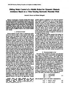
For most real-world applications, a mobile robot has to move within a dynamic environment. In this context, the problem is how to reach a target in the presence of dynamically moving obstacles. As seen above, when an obstacle is static, avoidance is accomplished by measuring its relative position. When an obstacle is moving, on the other hand, collision avoidance is harder because the robot has to detect not only the position but also the direction of the moving obstacle. In this experiment, the objective is to navigate the mobile robot to its goal in an unknown environment without any collisions with moving obstacles. During the first 7 time steps, both, the stimulus (Figure 7.3.b) as well as the field activation (Figure 7.3.a) are unimodal, since the stimulus contains only the target entries. In the following time steps, the stimulus contains the obstacle 1 entries. On the field activation, the peak changes its position according to the stimulus. Thus, the robot changes its direction (Figure 7.3.d) and slows down its speed (Figure 7.3.c). At time 16, the entries of the target becomes stronger than those of the obstacle. The peak change its position relative to the direction of the target. At time 18 the stimulus contains entries of obstacle 2. Again, the robot behaves with the same manner until it reaches the target. Figure 7.3.(e) shows the entire path movement of the robot.


120

55 50 Stimulus

2 Field Activation

1 0

45 40

−1

35

−2

60 50

−3 −4 60

30 60

40 30 50

40

60

40 40

20 30

20

10

20

10

Neurons

0

0

Time

20 0

Neurons

(a)

0

Time

(b)

3

160

2.5

140

120 Robot’s heading

Linear Velocity

2

1.5

100

80

1 60

0.5

0 0

40

10

20

30 Time

40

50

60

(c)

20 0

10

20

30 Time

40

(d)

(e)

Figure 7.2: Target acquisition with Obstacle avoidance

50

60


2

55

1

50

0

Stimulus

Field Activation

121

−1

45

40

−2 −3 60

35 60 80

40 20

80

40

60 40

60 40

20

20 0

Neurones

0

20 0

Neurones

Time

(a)

0

Time

(b)

2

100

1.8

80

1.6

60

1.4 Robot’s heading

Linear Velocity

40

1.2 1 0.8

20 0 −20

0.6 0.4

−40

0.2

−60

0 0

10

20

30

40

50

60

70

Time

−80 0

10

20

30

40

50

60

70

Time

(c)

(d)

(e)

Figure 7.3: Collision Avoidance for Moving Obstacles. The dotted lines in (e) represent the old positions of the obstacles.


122

Corridor Following The behavior Corridor-Following navigates the robot along an empty corridor. Two experiments are presented: in the first, the initial position of the robot is supposed to be in the middle between the corridor walls, as well as the target point. This is the simplest case, since it can be considered as a target acquisition with no obstacles. During the whole experiment, the field has only one peak on the heading direction 0o (Figure 7.4.a). This behavior is expected, since the stimulus contains only the target entries (Figure 7.4.b). Thus, the robot moves with the heading angle 0o until it reaches the target (Figure 7.4.e), and its velocity depends only on the distance relative to the target (Figure 7.4.c). In the second experiment, the robot starts from a position near a wall (Figure 7.5.e). In this case, the field is expected to guide the robot towards the target on the center of the corridor, with wall avoidance. In the first 14 time steps, the stimulus contains obstacle entries (Figure 7.5.b). Therefore, the field’s peak moves to an optimum provided by the stimulus (Figure 7.5.a). The robot moves with negative heading angles, until the behavior target-acquisition dominates the stimulus entries (Figure 7.5.d). Door Passing The behavior Door-Passing is supposed to navigate the robot to a target, but through a door. This is in principal the same behavior target-acquisition with obstacle-avoidance. However, the door has to be large enough, so that at the door, the stimulus entries will be dominated by the target acquisition. This is necessary to lead the robot through the door. Figure (7.6) shows the experiment result.


3

123

55

1

50 Stimulus

Field Activation

2

0 −1 −2

45

−3 −4 60

40 60 50

40 20 Neurones

50

40

40

40

30

20

20 10

0

0

30

Neurones

Time

(a)

20 10

0

0

Time

(b)

3

1 0.8

2.5 0.6 0.4 Robot’s heading

Linear Velocity

2

1.5

1

0.2 0 −0.2 −0.4 −0.6

0.5

−0.8

0 0

10

20

30

40

50

Time

−1 0

10

20

30 Time

(c)

(d)

(e)

Figure 7.4: Corridor Following: experiment 1

40

50

2

55

1

50

124

0 Stimulus

Field Activation


−1 −2

45 40 35

−3 −4 60

30 60 80

40 20

80

40

60 40

60 40

20

20 0

Neurones

0

20 0

Neurones

Time

(a)

0

Time

(b)

2

60

1.8 40

1.6 1.4 Robot’s heading

Linear Velocity

20

1.2 1 0.8

0

−20

0.6 0.4

−40

0.2 0 0

10

20

30

40

50

60

70

Time

−60 0

10

20

30

40 Time

(c)

(d)

(e)

Figure 7.5: Corridor Following: experiment 2

50

60

70


2

55

1

50

0

Stimulus

Field Activation

125

−1

45

40

−2 −3 60

35 60 80

40 20

80

40

60 40

60 40

20

20 0

Neurones

0

20 0

Neurones

Time

(a)

0

Time

(b)

2

100

1.8 80

1.6 60 Robot’s heading

Linear Velocity

1.4 1.2 1 0.8 0.6

40

20

0

0.4 −20

0.2 0 0

10

20

30

40

50

60

70

−40 0

10

20

Time

30

40 Time

(c)

(d)

(e)

Figure 7.6: Door Passing

50

60

70

7.5 Competitive Dynamics for Home-bases Acquisition

7.5

126

Competitive Dynamics for Home-bases Acquisition

Eilman and Golani [112] show by experiments that when rats are brought in a novel environment, they move alternately between stop and go. The place in which they stay for the longest time is defined as the rat’s home-base. In addition, it was observed, that when they want to reach a target, they prefer going through these home-bases instead of going through novel environments. These home-bases are typically installed only in areas, which are meaningful for them (e.g food places). In behavior control, this can be considered as an optimisation problem of planning reliable landmark-based robot navigation. A necessary condition for this optimization is that the generated path should be the shortest path through the maximum intermediate home-bases. Naturally, this must be not much longer than the direct way to the target. In this section, we adopt the concept of neural fields to optimize the target path through home-bases. The idea is to use an extra one-dimensional neural field, we call it sub-target neural field, that expresses, whether a home-base is the next sub-target or not. A Peak will decode the direction to a subtarget whenever one, or no peak otherwise. Following this method, the entire optimal trajectory from the start to the main target will be not necessary to be known, but only local information about the next sub-target. This implies also that the optimal decisions are not static: a change in the accessibility of a home-base leads to change the decision on which optimal home-base to visit next. To produce an optimal path planning, the sub-target neural field should produce a peak solution based on two requirements: a sub-target must be the nearest home-base to the robot and on the way to the main target, i.e. the shortest path to the main target (Figure 7.7.a), and flexibility: when for instance an obstacle forces the robot to make a detour, the path should be changed to another home-base (Figure 7.7.b). This makes a re-calculation of the optimization not necessary. Although the local decisions made by the two neural fields, the trajectory generated through all sub-targets will be the global optimal one, if no changes in the environment occur.


(a)

127

(b)

Figure 7.7: Sub-targets Acquisition

7.5.1

Sub-target Neural Field

This field has almost the same characteristics as the navigation field (7.10). It encodes home-bases angles from −π to π : τ u˙ ST (i, t) = −uST (i, t) + SST (i, t) + h +

N X

w(i, j)f [uST (j, t)]

(7.21)

j=1

where uST (i) is the field activation at the position i. A nonlinear interaction with its neighboring j positions is achieved by the convolution of an interaction kernel w(i, j). τ (τ ∈ R+ ) is the time constant. The constant h defines the pre-activation of the field, and f (uST ) is the local activation function. SST (i, t) is the external stimulus at the neuron i. Home-bases Stimulus As for navigation, the neural field (7.21) needs some necessary information (stimulus) about the home-bases locations. A home-base becomes a subtarget if it fulfills the requirement of being the nearest one to the robot and on the way to the main target. Thus, the stimulus is based on the location of the home-bases, on the position of the main target and on the current position of the robot. This stimulus is designed excitatory, showing


128

an attraction towards a sub-target. The stimulus of each home-base k is chosen as: (

SHBk (i, t) =

2

CHB (dT − dHBk )e−σHB (i−iHBk ) , dHBk < dT 0, dHBk ≥ dT

(7.22)

where CHB and σHB are positive constants, which depends on the field characterstics. dT and dHBk are the distances of the main target and the homebase k relative to the robot, respectively. The distance dHBk gives an advantage to the home-bases, which lie closer to the robot. However, the term CB (dT − dBk ) alone is not enough, because the generated trajectory may not be the globally optimal. It may lead to detours, which violate the requirement of shortening the path. To prevent this, a Mexican Hat function 2 (e−σST (i−iT ) ), centred at the direction of the main target iT , is used to eliminate the effect of all home bases, which are not on the way to the main target. Furthermore, obstacles must be taken into consideration, in order to change the plan if necessary. The global stimulus of the Sub-target neural field is the contribution of all home bases stimulus. Thus the global stimulus at time t will be: SST (i, t) =

X

2

SHBk (i, t)e−σST (i−iT ) −

k

7.5.2

NX Obst

g(dOl )SOl (i, t)

(7.23)

l=1

Target-acquisition Stimulus

To acquire these sub-targets, the stimulus of the navigation neural field (7.15) must be modified. When a sub-target is localized, the robot should move to it and ignore the attraction of the main target. Thus the influence of the main target is switched off, and the active sub-target errects a peak solution. When an obstacle is detected or no sub-target is active, the main target is acquired. These requirements can be reached by the modification bellow: S(i, t) = (1 − HV (uST ))(ST (i, t) −

NX Obst

g(dOl )SOl (i, t)) + HV (uST )SST (i, t)

l=1

(7.24)

where HV (.) is the heavside function: (

HV (uST ) =

1, uST > 0 0, uST ≤ 0

(7.25)


7.5.3

129

Results

The sub-target neural field has the same number of neurons (NST = 60). We consider that the position of a home-base in the spatial coordinates is (XHB , YHB ). From the actual position of the robot (Xr , Yr ), the angle to a home-base is: YHB − Yr ) (7.26) ϕHB = arctan( XHB − Xr The main target is acquired by planning optimal sequences through the intermediate home-bases. Figure (7.8) illustrates a first experiment. In the first 20 time steps, the sub-target field selects, through competition, the home-bases 1 and 3 to be intermediate sub-targets to the main target (Figure 7.8. b). In the following time steps, it can be seen that when there is no sub-targets on the target way, the main target is acquired. This result demonstrates that the first requirement of shortening the target path, mentioned earlier, is fulfilled. The second requirement of flexibility is tested in the next simulation. Figure (7.9) shows the case, where the robot should avoid an obstacle. We repeat the same experiment above, but an obstacle is added on the way to the home bases 1 and 3. When the obstacle is detected, the influence of the home base 1 is switched off, and then only the main target is acquired with obstacle avoidance. After this detour, the home-bases 1 and 3 are not any more sub-targets. Instead, the home base 2 has the more advantage to be a sub-target, which is interpreted by switching ON the sub-target field. After passing the home-base 2, the main target is acquired.


4

130

120

80 Stimulus

Field Activation

100 2

0

60 40

−2 20 −4 60

0 60 50

40 20 Neurones

50

40

40

40

30

20

20 10

0

0

30

Neurones

Time

20 0

2

70

1.8

65

1.6

60

1.4

55

1.2 1 0.8

50 45 40

0.6

35

0.4

30

0.2

25

0 0

10

20

Time

(b)

Robot’s heading

Linear Velocity

(a)

10 0

30

40

50

20 0

10

20

30 Time

Time

(c)

(d)

(e)

Figure 7.8: Sub-target Acquisition Through Competition

40

50

4

150

2

100 Stimulus

Field Activation


0

−2

131

50 0 −50

−4 60

−100 60

60

40

60

40

40 20

40 20

20 0

Neurones

0

20 0

Neurones

Time

(a)

0

Time

(b)

2

80

1.8

70

1.6


Linear Velocity

1.4 1.2 1 0.8

50 40 30

0.6

20 0.4

10

0.2 0 0

10

20

30 Time

40

50

60

(c)

0 0

10

20

30 Time

(d)

(e)

Figure 7.9: Sub-targets Acquisition: Flexibility

40

50

60

7.6 Neural Fields for Multiple Robots Control

7.6

132

Neural Fields for Multiple Robots Control

Recently, there has been increased research interest in systems composed of multiple mobile robots exhibiting cooperative behavior. Such systems are of interest for several reasons: i) tasks may be too complex (or impossible) for a single robot to accomplish, and ii) using several simple robots can be easier, cheaper, and more flexible than having a single powerful robot for one task. This is inspired from the nature. Living in a group provides animals to combine their sensors to maximize the chance of detecting predators, or searching for food. A key problem in cooperative robotics is to maintain a certain geometric configuration during movement. The reason is that there are many interesting tasks that require multiple robots to coordinate their movements for example box-pushing [113], and movement of a team of military robotic vehicles as a scout unit [114]). There are two main ways of approaching this problem: model-based control, and behavior-based control. In the first, the objective is to build a model for the team of robots and the desired task, and develop a framework to optimise their performance [115]. This method has a limit success when the robots behave in a dynamic and unknown workspace. By contrast, in behavior-based control no model is required. The control system is in a form of reactive behaviors to the current state of the environment [114]. In this section we investigate how neural fields can produce an elegant solution for the problem of moving in formation. The objective is to acquire a target, avoid obstacles and keep a geometric configuration at the same time. Several formations for a team of three robots are considered (Figure 7.10): . line: robots move line-abreast, . column: robots move one after the other, . triangle: robots move in a triangle formation. The strategy is to have a leader (robot 1) guiding followers (robots 2 and 3). The robots should avoid obstacles and collisions among them. We assume that the robots are identical, and dont fail during travel.


(a)

(b)

133

(c)

Figure 7.10: Geometric Configurations: a) line, b) column, c) triangle

7.6.1

Control Design

Each robot 1, 2, and 3 has its own neural field model. We choose the robots’ headings ϕk (k ∈ {1, 2, 3}) relative to a world-fixed reference direction as behavioral variables. Hence, each neural field has to encode angles from −π to +π. By means of a codebook we use N discrete directions. The three neural field models will be described by: τ u˙k (i, t) = −uk (i, t) +

N X

w(i, j)f [uk (j, t)] + Sk (i, t) + h

(7.27)

j=1

where k ∈ {1, 2, 3}. Each interaction kernel is chosen as: 2

w(i, j) = kw e−σw (i−j) − H

(7.28)

where the parameter σw and kw are used to adjust the range of excitation and its amplitude, respectively. The global inhibition H allows only one localized peak on the field. After the stabilization of the field, the most activated neuron decodes the direction to be executed by a robot: ϕF = argmax {u(i)|i ∈ [1, N ]}

(7.29)

Before selecting an appropriate direction of a robot, each neural field needs some necessary information (stimulus).


7.6.2

134

Field Stimulus

Based on the tasks described earlier, the stimulus is determined according to two stimulus-functions. These functions describe: 1 the direction towards the target. This stimulus is designed excitatory, showing an attraction to the desired direction of each robot. The target of the leader is the “main target”. Thus, its stimulus can be chosen as: ST leader (i, t) = CT 1 − CT 2 |i − imain (t)|

(7.30)

where CT 1 , CT 2 are constants positive, and imain (t) is the field position, equivalent to the main target direction at time t. The followers are attracted by the required configuration relative to the leader. In this case each follower has the target stimulus : ST k (i, t) = CT 1k − CT 2k |i − iT k (t)|

(7.31)

where CT 1k , CT 2k are constants positive, and iT k (t) is the field position, equivalent to the direction of the required position of the robot k (k ∈ {2, 3}) at time t. 2 the directions to obstacles {SOl (i, t) : l ∈ [1, NObst ]}, where NObst are the number of obstacles detected by the robot sensors. This stimulus must be inhibitory, since obstacles collision must be avoided. It is chosen as a Mexican Hat function centered at the direction of an obstacle. SOl (i, t) = CO e−σO (i−il )

2

(7.32)

where CO and σO are positive constants. σO defines the range of inhibition of an obstacle. In practical situations, this parameter is tuned regarding the radius of the robot and the obstacles. il reflects the direction of the obstacle l at time t. Obstacles here include also other robots, since they should avoid collision among tem. However, the stimulus consider only obstacles, which their distances dOl to the robot are less than a threshold dT h . Thus, the global obstacle stimulus is determined by: SO (i, t) =

NX Obst l=1

g(dOl )SOl (i, t)

(7.33)


135


g(d) =

1, d < dT h 0 d ≥ dT h

(7.34)

Using the step function g, only obstacles , which their distances dOl to the robot are less than a threshold dT h , are considered. The contributions of different stimulus define the global stimulus for each neural field. For the leader neural field, the stimulus at time t is determined by Sleader (i, t) = ST leader (i, t) − CM SO (i, t) (7.35) For the followers, the stimulus is: Sk (i, t) = ST k (i, t) − CM SO (i, t)

(7.36)

where k ∈ {2, 3}, and CM is a constant positive.

7.6.3

Formation Control

For each configuration, two tasks, formation-speed and formation-steer run simultaneously to maintain each robot in its desired position. formation-speed In a free obstacle situation, the leader moves with its maximum speed Vmax , and slows down when it approches a target. This dynamics can be chosen as: VT (t) = Vmax (1 − e−σv dT ) (7.37) where σv is a constant tuned in a relation with the acceleration capability of the robot, and dT represents the distance between the robot and the target at time t. When it approaches obstacles, its velocity must be reduced. This dynamics can be chosen as: 2


(7.38)

where CO and σOv are constant. inO is the nearest obstacle direction to the robot movement direction, and dnO is its distance relative to the robot. The final dynamics of the leader velocity is the contribution of (7.37) and


136

(7.38). It is also considered when no appropriate direction can be selected, for example when the robot is completely surrounded by obstacles. In this case the robot must stop until the environmental situation changes. Thus, the global leader velocity that satisfies the above design creteria is the following: (

Vleader (t) =

VT (t)VO (t), ϕF > 0 0 ϕF ≤ 0

(7.39)

The following steps summarize how a follower selects its speed: . If a follower is behind its desired position, it should speed up. . If a follower is in front of its desired position, it should slow down. In presence of obstacles, the speed is slowed down, depending on the distance to the obstacle. This speed dynamics can chosen as follows: (

Vk (t) =

(Vleader (t) + p|δspeed |)VO (t), ϕF > 0 0 ϕF ≤ 0

(7.40)

where p is a positive constant parameter used to adjust the rate of correction, and δspeed ∈ [−1, +1] is the correction term. Its value varie depending on how far a follower from its desired position is. formation-steer According to figure (7.11), desired positions for the configurations line and traingle are: (

(

x2 = xleader + dist2 sin(θleader − α2 ) y2 = yleader − dist2 cos(θleader − α2 )

(7.41)

x3 = xleader − dist3 sin(θleader + α3 ) y3 = yleader + dist3 cos(θleader + α3 )

(7.42)

where dist2 and dist3 are the distances of the followers 2 and 3 relative to the leader, respectively. In the case of line formation, α2 = 0 and α3 = 0. For the column formation (Figure 7.12) , desired positions are: (

x2 = xleader − dist2 cos(θleader ) y2 = yleader − dist2 sin(θleader )

(7.43)

7.6 Neural Fields for Multiple Robots Control (

x3 = xleader − dist3 cos(θleader ) y3 = yleader − dist3 sin(θleader )

Figure 7.11: Triangle and Line Configuration

Figure 7.12: Column Configuration

137

(7.44)

7.7 Results

7.7

138

Results

In order to update the field stimulus, we assume that each robot has a 360o sensor. The sensor range is assumed to be a circle with a radius equal to 1. On each neural field we chose N = 60 neurons, which means that each direction N decodes a step of 6o . Figure (7.13) shows a simulation run, where the objective is to maintain the line-abreast formation. At the beginning the followers started with a higher speed, in order to reach the desired position, since they started away from the leader (Figure 7.13 a). Once the required positions are reached, they move with the same heading and speed of the leader. The next simulations evaluate the obstacle-avoidance and maintainformation performance. Figures (7.14) and (7.15) show the obtained results for avoiding obstacles and acquiring static and moving targets. When a robot is close to an obstacle, the stimulus contain obstacle entries, which brought the robot away from the obstacle. This behavior was expected, since obstacle-avoidance behavior has the highest priority. The same behaviors can observed on figures (7.16), (7.17) and (7.18) for the formation triangle. The result of colmun formation are presented in Figure(7.19). colmun formation is also tested in the case of door passing (Figure 7.20). In this test, the control approach has succefully provided the robots the ability to traverse through a narrow gap, and maintaining the colmun formation.

7.7 Results

139 150 Leader Follower 2 Follower 3

Robots headings

100

50

0

−50

−100

−150 0

5

10 Time

15

20

(a) 3.5 Leader Follower 2 Follower 3

3

Linear Velocities

2.5

2

1.5

1

0.5

0 0

5

10 Time

15

20

(b)

(c)

Figure 7.13: Line configuration in obstacle free situation. a)Robots’ headings. b) Robots’ velocities

7.7 Results

140 80 60

Robots headings

40 20 0 −20 −40 −60 −80 0

5

10

15

20

25

15

20

25

Time

(a) 3.5

3

Linear Velocities

2.5

2

1.5

1

0.5

0 0

5

10 Time

(b)

(c)

Figure 7.14: Line configuration with obstacles. a)Robots’ headings. b) Robots’ velocities

7.7 Results

141 80 60

Robots heading s

40 20 0 −20 −40 −60 −80 0

5

10

15

20

25

15

20

25

Time

(a) 3.5

3

Linear Velocities

2.5

2

1.5

1

0.5

0 0

5

10 Time

(b)

(c)

Figure 7.15: Line configuration with moving target and fixed obstacles. a)Robots’ headings. b) Robots’ velocities

7.7 Results

142 150

Robots headings

100

50

0

−50

−100

−150 0

5

10

15

20

25

20

25

Time

(a) 3

Linear Velocities

2.5

2

1.5

1

0.5

0 0

5

10

15 Time

(b)

(c)

Figure 7.16: Triangle configuration. a)Robots’ headings. b) Robots’ velocities

7.7 Results

143 100

Robots’ heading

50

0

−50

−100

−150 0

2

4

6

8

10

12

14

10

12

14

Time

(a) 3

Linear Velocity

2.5

2

1.5 0

2

4

6

8 Time

(b)

(c)

Figure 7.17: Triangle configuration with moving target. a)Robots’ headings. b) Robots’ velocities

7.7 Results

144 100

Robots’ heading

50

0

−50

−100

−150 0

5

10

15 Time

20

25

30

20

25

30

(a) 3

Linear Velocity

2.5

2

1.5

1

0.5 0

5

10

15 Time

(b)

(c)

Figure 7.18: Triangle configuration with moving target and fixed obstacles. a)Robots’ headings. b) Robots’ velocities

7.7 Results

145 3.5

3

Linear Velocity

2.5

2

1.5

1

0.5

0 0

5

10 Time

15

20

15

20

(a) 80 60 40

Robots’ heading

20 0 −20 −40 −60 −80 −100 0

5

10 Time

(b)

(c)

Figure 7.19: Column configuration in a door passing test. a)Robots’ headings. b) Robots’ velocities

7.7 Results

146 3

2.5

Linear Velocity

2

1.5

1

0.5

0

−0.5 0

5

10

15

20

25

30

35

20

25

30

35

Time

(a) 150

100

Robots’ heading

50

0

−50

−100

−150 0

5

10

15 Time

(b)

(c)

Figure 7.20: Column configuration in a door passing test. a)Robots’ headings. b) Robots’ velocities

7.8 Conclusion

7.8

147

Conclusion

In this chapter, neural fields have been chosen as a framework for the behavior based robot control. While their suitability has been already proven to solve the problem of target-acquisition with obstacle avoidance [110][111], we described here how neural fields could be used in more complex problems: avoiding static and moving obstacles, multi-target acquisition, and maintaining formation for multiple robots. The navigation model is developed in order to produce peak-solutions of the field activation, which encode the appropriate robot direction in response to a change in the environment. Through competitive dynamics, the sub-target neural field expresses, whether a homebase is the next sub-target or not. A Peak will decode the direction to a sub-target whenever one, or no peak otherwise. Following this method, the entire optimal trajectory from the start to the main target was not necessary to be known, but only local information about the next sub-target. This implies that the optimal decisions were not static: a change in the accessibility of a home-base leaded to change the decision on which optimal home-base to visit next. For multirobot control, we have decomposed the problem of formation control into: 1) control of a single lead robot and 2) control of two follower robots in the team. The lead robot has to acquire the main target, while the follower robots maintain formation. In addition, all robots have to avoid obstacles and collision with each other. Based on these requirements, the three neural fields were provided by the necessary stimulus information. Three geometric configurations were considered: line, column, and triangle. For each configuration, two tasks, formation-speed and formation-steer run simultaneously to keep each robot in its desired position. Simulations results demonstrate the smooth behavior of the robots, despite all imposed constraints. Figure (7.18) demonstrates that tracking a moving target, avoiding obstacles, and maintaining triangle formation is not an absolute limitation of our approach. The scenario of passing a door in a column formation did not present any difficulty as well (figure (7.20)). Furthermore, in all developments, the speed control is fully integrated here. In earlier studies, this quantity was usually set to a constant value. All in all, simulations results demonstrate that the neural field concept could provide an elegant solution for behavior-based control of single or multiple mobile robots, despite many imposed constraints. A real implementation of the control design will be presented in chapter (8).

Chapter 8 Neural Fields for Behavior-Based Control of a RoboCup Player As seen in previous simulation results, neural fields provide an elegant local solution for behavior control. Due to their low-computational costs, this approach is suitable for real application where the environmental state changes continually. This chapter presents a set of experiments in a real environment. The main objective is to move a robot to a target while avoiding static and moving obstacles. Experimental tests were obtained using the same robot (figure 8.1) used in chapter (6).

(a)

(b)

Figure 8.1: Omnidirectional robot. a)hardware photo. b) CAD model

8.1 Robot System

8.1

149

Robot System

The neural field approach is implemented on one robot of the CoPS-Team (Cooperative Soccer Playing Robots) of Stuttgart University [116]. It is equipped with 3 omni-wheels, each of them driven by a 90W DC motor. Gearboxes with reduction ratios of 14:1 are used to reduce the high angular speeds of the motors (7000 rpm) and to amplify the wheel’s mechanical torques, and 500 ppr digital incremental encoders are used to measure the actual wheels speed. Motors are controlled by 3-channel microprocessor-based interface. The robot is equipped with a laptop to manage different sensors and tasks. The communication between the sensors and the laptop can be done through USB, RS232, or IEEE1394 (FireWire). A pneumatic kicker supplied by a small air pressure tank is also installed on the robot.

8.1.1

Environment Sensing

For environment sensing, the robot platform is equipped with an omnidirectional vision system, based on a hyperbolic mirror and a standard IEEE1394 (FireWire) camera. The Omnidirectional vision provides the robot a very large field of view, which has some useful properties. For instance, it can facilitate the tracking of robots, the ball, and a set of environmental features used for self-localization. To extract information, the captured image is segmented using the calibrated colors of relevant objects, such the ball, field lines, and obstacles. An example of an image with recognized objects is shown in Figure (8.2).

8.1 Robot System

150

(a)

(b)

Figure 8.2: Information extraction from the camera a) Image captured from the omni-camera b) Recognition of relevant objects: lines(white), ball(red), obstacles (black), and goals (blue and yellow).

8.1.2

Self-Localization

The problem of self-localization is to estimate the robots pose relative to its environment. In our robots we use a probabilistic localization algorithm called Monte Carlo Localization (MCL) [117]. MCL can solve the localization problem in a highly robust and efficient way, even with temporary partial or total occlusion of relevant sensor features.

8.1.3

Software Architecture

The Software architecture has a modular design structured into three parallel working layers (Figure 8.3): 1 Sensor layer, where low level features or raw data are gathered, 2 World Model layer, which is used for storage and administration of data objects. It provides so-called Data Processor modules. These modules work on dedicated data objects of the world model to generate data of a higher degree of abstraction. Monte Carlo based localization and Kalman filter based ball tracking are examples of theses modules. The

8.2 Neural Fields

151

world model stores locally gathered data as well as communicated data by other robots. 3 Control layer, responsible for the execution of actions. While its Pilot module simply provides driving and steering capabilities, its Navigator module implements complete soccer behaviors like driving or dribbling to a position or shooting a ball.

Figure 8.3: Robot Software Architecture.

8.2

Neural Fields

For convinient, we rewrite the field equation of a one-dimensional neural field: τ u(ϕ, ˙ t) = −u(ϕ, t) + S(ϕ, t) + h +

Z +∞ −∞

w(ϕ, ϕ)f ´ (u(ϕ, ´ t)dϕ´

(8.1)

where u(ϕ, t) is the field excitation at time t (t ≥ 0) at the position ϕ ∈ R. The temporal derivative of the excitation is defined by u(ϕ, ˙ t) =

∂u(ϕ, t) ∂t

(8.2)

The excitation u(ϕ, t) of the field varies with the time constant τ with τ ∈ R+ . The constant h defines the pre-activation of the field, and f (u) is the local activation function. Usually, f is chosen as a step-function: (

f (u) =

1, u ≥ 0 0 u −h. 3. There exists an a-solution (a local excitation of length a) if and only if h < 0 and a > 0 satisfies W (a) + h = 0. 4. The a-solution is asymptotic stable if

dW (a) da

< 0, and unstable if

dW (a) da

> 0.

8.3 Control Design

153

As seen in chapter (7), if the field is in a-solution and an input of a stimulus S(i, t) at time t is very large compared with the within-field cooperative interaction, this input will dominate the solution. As a result, a single-peak will be stabilized by interaction, even if the stimulus is removed.

8.3

Control Design

In the experiments, the neural field has to encode angles from −π to +π. By means of a codebook we use N discrete directions. The one-dimensional neural field for the robot directions will be: 

τ u(i, t + ∆t) = (τ − ∆t)u(i, t) + ∆t 

N X



w(i, j)f [u(j, t)] + S(i, t) + h (8.8)

j=1

The neural parameters field are chosen as follows. The pre-activation h of the filed is fixed to h = −1, the time constant to τ = 2, and the discret time ∆t = 0, 2. The interaction kernel is chosen as: 2

w(i, j) = 5e−0.5(i−j) − 2

8.3.1

(8.9)

Field Stimulus

Before selecting an appropriate robot direction, the neural field needs some necessary information (stimulus). The stimulus is determined according to two stimulus-functions. These functions describe 1 the direction towards the target ST (i, t). This stimulus is designed excitatory, showing an attraction towards the target direction. It is chosen as ST (i, t) = CT 1 − CT 2 |i − iT (t)| (8.10) where CT 1 = 25, CT 2 = 1, and iT (t) is the field position, equivalent to the target direction at time t. 2 directions to obstacles {SOl (i, t) : l ∈ [1, N ]}, where NObst are the number of obstacles detected by the robot sensors. However, the stimulus consider only obstacles, which their distances dOl to the robot are less than

8.3 Control Design

154

a threshold dT h = 1m. This stimulus must be inhibitory, since obstacles collision must be avoided. It is chosen as a Mexican Hat function centered at the direction of an obstacle. SOl (i, t) = CO e−σO (i−il )

2

(8.11)

where CO = 50,and σO = 0.05 which defines the range of inhibition of an obstacle. The contribution of different stimulus defines the state of the field. Thus, the stimulus of the field at time t is determined by S(i, t) = ST (i, t) −

NX Obst

g(dOl )SOl (i, t)

(8.12)

l=1


g=

8.3.2

1, dOl < dT h 0 dOl ≥ dT h

(8.13)

Dynamics of Speed

In a free obstacle situation, the robot can move with its maximum speed Vmax = 1.5m/s. However, close to obstacles or a target the robot needs to be slowed down. In free obstacles, the velocity can be chosen as: VT (t) = Vmax (1 − e−σv dT )

(8.14)

where σv = 0.8, and dT represents the distance of the robot relative to the target at time t. When the robot approaches obstacles, its velocity must be reduced relative to the obstacle distance and its direction. In case of many obstacles, the nearest obstacle direction to the robot movement direction is considered. This dynamics can be chosen as: 2


(8.15)

where CO = 1 and σOv = 0.003. inO is the nearest obstacle direction to the robot movement direction and dnO is its distance relative to the robot. The final dynamics of the velocity is the contribution of (8.14) and (8.15). Furthermore, it is also considered when no appropriate direction can be selected, for example when the robot is completely surrounded by obstacles.

8.4 Results

155

In this case the robot must stop until the environmental situation changes. Thus, the robot velocity that satisfies the above design creteria is the following: ( VT (t)VO (t), ϕF > 0 (8.16) V (t) = 0 ϕF ≤ 0

8.4

Results

Expriments were made on a soccer field of 10, 421m length and 5, 720m width. The origin of the coordinates is taken on the middle of the field. On the neural field we chose N = 60 neurons, which means that each direction N decodes a step of 6o . In all experiments, the initial and the target positions of the robot are given in the spatial coordinates and equal to (−3000, 0), (3000, 0), respectively. The neural field is expected to align the robot’s heading with the direction of the target, and to bring it away from the nearby obstacles. We will illustrate this with some experiments showing target acquisition with collision avoidance for multiple static and moving obstacles. Figure (8.4) shows the results of the first experiment. In the first 20 time steps, both, the stimulus (Figure 8.4.b) as well as the field activation (Figure 8.4.a) are unimodal, since no obstacles are detected and the stimulus contains only the target entries. In the following time steps, the stimulus contains also obstacle entries. Therefore, it becomes bimodal. By contrast, on the field activation, the peak follows the optimum direction produced by the targetacquisition and obstacle-avoidance behaviors. It provides now the appropriate heading direction towards the target with obstacle avoidance (Figure 8.4.d). We can see also how the robot speed is slowed down when it is near the obstacle or approaches the target (Figure 8.4.c). In this experiment, the distance between the obstacles 2 and 3 is not enough to contain the robot dimension. Due to the contribution of the two obstacle stimulus the robot was obliged to pass to the right and avoid obstacle 3 in order to reach the target. Figure (8.4.e) shows the entire path movement of the robot from its initial position to the target position. Photos from video sequences are presented in figure (8.6). In the second experiment (figure 8.5), the distance between the obstacles 2 and 3 is now large enough to contain the robot dimension. The robot could move through these two obstacles to reach the target. Figure (8.7) shows some photos from video sequences of the second experiment. The third experiment (figure 8.8) was carried out to verify the navigation

8.4 Results

156

approach ability in tackling moving obstacles. In this context, the problem is how to reach a target in the presence of dynamically moving obstacles. During the first 20 time steps, both, the stimulus (figure 8.8.b) as well as the field activation (figure 8.8.a) are unimodal, since the stimulus contains only the target entries. In the following time steps, the robot avoids the obstacle 1. At time step 51, the stimulus contains obstacle 2 entries. In the next 15 time steps, the neural field provides the appropriate heading direction towards the target with obstacle 2 avoidance (Figure 8.8.d). After passing obstacle 2, the entries of the target became stronger. The peak changed its position towards the direction of the target. Figure (8.8.e) shows the whole path movement of the robot.

8.4 Results

157

4

40

20 0 Stimulus

Field Activation

2

−2 −4

0

−20 −6 −8 60

−40 60 80

40 20

80

40

60 40

60 40

20

20 0

Neurones

0

20 0

Neurones

Time

(a)

0

Time

(b)

2

200

1.8 150

1.4


Linear Velocity (m/s)

1.6

1.2 1 0.8

50

0

0.6 −50

0.4 0.2 0

10

20

30

40 Time

50

60

70

80

(c)

−100 0

10

20

30

40 Time

50

60

70

80

(d)

(e)

Figure 8.4: Target acquisition with Obstacle avoidance: first experiment

8.4 Results

158

5

40

Stimulus

Field Activation

20 0

−5

0 −20 −40

−10 60

−60 60 80

40

80

40

60

60

40

20

40

20

20 0

Neurones

0

20 0

Neurones

Time

(a)

0

Time

(b)

2

200

1.8 150

1.4



1.6

1.2 1 0.8

50

0

0.6 −50

0.4 0.2 0

10

20

30

40

50

60

70

Time

−100 0

10

20

30

40

50

60

70

Time

(c)

(d)

(e)

Figure 8.5: Target acquisition with Obstacle avoidance: second experiment

8.4 Results

Figure 8.6: Photos from video sequences of the first experience.

Figure 8.7: Photos from video sequences of the second experience.

159

8.4 Results

160

40

4

20

0

Stimulus

Field Activation

2

−2

0 −20

−4

−40

−6

−60 60

−8 60 200

40

200

40

150

150

100

20

100

20 50

50 0

Neurones

0

0

Neurones

Time

(a)

0

Time

(b)

1

200

0.9 150 100

0.7 Robot’s heading


0.8

0.6 0.5 0.4

50 0 −50

0.3 −100

0.2 −150

0.1 0 0

20

40

60

80 Time

100

120

140

160

(c)

−200 0

20

40

60

80 Time

100

120

140

(d)

(e)

Figure 8.8: Target acquisition with moving obstacle avoidance

160

8.5 Conclusion

8.5

161

Conclusion

In this chapter, we have demonstrated how neural fields have been chosen as a framework for the behavior-based control of a RoboCup Player. The navigation model is developed in order to produce peak-solutions of the field activation, which encode the appropriate robot direction in response to a change in the environment. The robot had to acquire the main target, while avoiding static and moving obstacles. This chapter demonstrated the utility of the approach only on one robot. One issue that needs to be addressed in future research is to implement the approach on multiple robots. In RoboCup, formation control plays a major role. For example, if a lead robot loss the ball, the other follower robots could catch it and continue the movement. Another application is in the defense position, where the robots should form a “wall” around the goal area.

Chapter 9 Conclusions and future work

9.1

Summary of Contributions

When we started this work, we had two goals: explore recurrent neural networks, and develop solutions for two robotics problems. We studied the idea that a large recurrent network can serve as a source of dynamics from which information can be extracted by a readout unit. It was adopted as a solution to overcome some RNNs training difficulties. Also, we explored the concept of metalearning to train a RNN that can adapt without changing explicit weights. Regarding robotics, we firstly designed a motion control approach based on a novel random recurrent neural network called echo state network (ESN). The advantage is that no knowledge about the robot model is required, and no synaptic weight changing is needed in presence of parameters variation. In addition, this ability allowed a single fixed weight ESN to act as a dynamic controller for several distinct mobile robots. In behavior-based control, the concept of neural fields theory was adopted to generate the robot behavior over time. We described how neural fields could be used to move a robot towards a target while avoiding static or moving obstacles. The naviga-

9.2 Conclusions

163

tion model was developed in order to produce peak-solutions of the field activation, which encode the appropriate robot direction in response to environment changes. Through their competitive dynamics, we also designed a framework to optimize the target path through intermediate home-bases. Moreover, we have demonstrated how neural fields are able to generate behavior control for multiple mobile robots. The objective was to move a team of robots to a target while avoiding obstacles and keeping a geometric configuration.

9.2

Conclusions

In this thesis we investigated how dynamics in recurrent neural networks can be used to solve some specific mobile robot problems. The ability of RNNs to handle arbitrary temporal dynamics, and robustness for noise environment make them an ideal choice for real dynamical systems control. However, this potential is not being exploited because simple and powerful training algorithms were missing. To overcome this problem we adopted the concept of echo state networks (ESNs). ESN has an easy training algorithm where only the network-to output connection weights have to be trained using a linear regression. The training experiments carried out here demonstrate that small and partially interconnected ESNs could be trained to act as motion controllers for mobile robots. Moreover, ESNs were being asked to deal with parameters variation. In other words, they were asked to exhibit a characteristic, normally ascribed to adaptive controllers, whose parameters change in response to an environmental change. “Adaptation” in this work is defined as the ability of an ESN to recognize change only through the system output and its own state, without changing any synaptic weight. This capability is a natural consequence of prior metalearning used during training. When a change occurred, the state of ESN switched from one family of orbits to another, which corresponds to the change. This ability allowed us also to design a single fixed-weight controller for multiple distinct mobile robots. The fixed-weight solution adopted here presents a clever and efficient strategy compared with adaptive networks. Furthermore, no multi-streaming is needed during training, since ESNs use a batch-learning algorithm and do not suffer from the recency effect. Neural fields have been chosen as a framework for the behavior-based

9.3 Future Directions

164

control. While their suitability has been already proven to solve the problem of target-acquisition with obstacle avoidance, we described here how they could be used in more complex problems: acquiring one or multiple targets, avoiding static and moving obstacles, and maintaining formation for multiple robots. The navigation models were developed in order to produce peaksolutions of the field activation, which encode the appropriate robot direction in response to a change in the environment. The entire optimal trajectory from the start to the main target was not necessary to be known, but only local information was needed. This implies that the optimal decisions were not static: a change in the accessibility of a home-base for example leaded to change the decision on which optimal home-base to visit next. In multi-robot control, two behaviors, formation-speed and formation-steer run simultaneously to keep each robot in its desired position. The obtained results demonstrate the smooth behaviors, despite all imposed constraints. All in all, we have shown that dynamics in RNNs could provide simple and elegant solutions for some problems in mobile robotics. Successful results have been obtained on simulations and on real implementations. However, several open issues still remain for future research.

9.3

Future Directions

Although we consider that the objectives of this thesis have been accomplished, there are plenty of improvements that could be done in order to achieve better results. Here, only the main points are summarized. • We are aware of a certain degree of arbitrariness in our choice of the ESN parameters and architecture. Substantial investigation and more experiments on much larger data sets are still needed to ensure that the results we have achieved to date are indeed statistically significant. • How to guaranty stability? As any RNN, a relatively large dimension ESN lost stability at many times and exhibited sometimes highfrequency oscillations on smooth test signals. • What is the behavioral capacity of RNNs? In this work, we explored the performance of ESNs to exhibit adaptive behavior with fixed-weights.

9.3 Future Directions

165

However, we did not discuss the question whether the obtained fixedweights ESNs could pass any test in adaptive system. Our network works well only for those situations, for which it has been trained. This may be seen as a limitation relative to explicitly adaptive systems. Does a more efficient training method exist? • We have provided a control framework based on neural fields theory. Much more efforts must be done to completely integrate movement planning and motor control. One important issue is to integrate the speed control with the temporal evolution of neural activation. A first step towards addressing this issue is to find out what are the optimal neurons activation states before and after performing movements. Further step is to estimate the optimal timing of the movement. • Only simulation results demonstrated the neural fields utility for multirobot system. This approach must be implemented and tested on a team of real robots (for example a team of RoboCup robots).

Bibliography [1] Mataric Maja J. Behavior-based control: Examples from navigation, learning, and group behavior. Journal of Experimental and Theoretical Artificial Intelligence, special issue on Software Architectures for Physical Agents, 9:323–336, 1997. [2] Erann Gat. On three-layer architectures. Artificial Intelligence and Mobile Robots,MIT/AAAI Press, 1997. [3] Connell Jonathan. A hybrid architecture applied to robot navigation. In Proc. of the 1992 IEEE International Conf. on Robotics and Automation, pages 2719–2724, 1992. [4] Arkin R. Towards the unification of navigational planning and reactive control. In American Association for Artificial Intelligence Spring Symposium on Robot Navigation, pages 1–5. AAAI/MIT Press, 1989. [5] Brooks Rodney A. A robot that walks; emergent behavior from a carefully evolved network. Neural Computation, pages 253–262, 1989. [6] Connell Jonathan. Designing behavior-based robots. In SPIE-91 Conference on Mobile Robots, volume 1613, pages 34–45, 1991. [7] Brooks Rodney A. A robust layered control system for a mobile robot. IEEE Journal of Robotics and Automation, 2(1):14–23, Mar 1986. [8] Brooks Rodney A. New approaches to robotics. Science, 253:1227– 1232, 1991. [9] Mataric Maja J. Navigating with a rat brain: a neurobiologicallyinspired model for robot spatial representation. In First International Conference on Simulation of Adaptive Behavior, pages 169–175, Cambridge,MA, 1990. MIT Press.

BIBLIOGRAPHY

167

[10] Mataric Maja J. Integration of representation into goal-driven behavior-based robots. IEEE Transactions on Robotics and Automation, 8(3):304–312, 1992. [11] Pirjanian P. Multiple Objective Action Selection and Behaviour Fusion using Voting. PhD thesis, Aalborg University, 1998. [12] Jana Kosecka and Ruzena Bajcsy. Discret event systems for autonomous mobile agents. In Proceedings of Intelligent Robotic Systems, pages 21–31, July 1993. [13] Long-Ji Lin. Scaling up reinforcment learning for robot control. In Proceedings of the 10th International Conference on Machine Learning, 1993. [14] Steen Kristensen. Sensors Planning with Bayesian Decision Analysis. PhD thesis, Department of Medical Informatics and Image Analysis, Aalborg University, 1996. [15] Pirjanian P. Behavior coordination mechanisms – state-of-the-art. Technical Report IRIS–99–375, Institute of Robotics and Intelligent Systems, School of Engineering, University of Southern California, 1999. [16] Payton D., Kersey D., Kimble D., Krozel J., and Rosenblatt K. Do whatever works: A robust approach to fault-tolerant autonomous control. Applied Intelligence, 3:226–249, 1992. [17] Saffiotti A., K. Konolige, and E. H. Ruspini. A multivalued-logic approach to integrating planning and control. Artificial Intelligence, 76(12):481–526, 1995. [18] Hoffmann Frank. An overview on soft computing in behaviour based robotics. In Proc. Joint 10th IFSA World Congress, Istanbul, Juni 2003. [19] Hoffmann Frank. Fuzzy behavior coordination for robot learning from demonstration. In NAFIPS 2004, Banff Canada, June 2004. [20] O. Khatib. Real-time obstacle avoidance for manipulators and mobile robots. International Journal of Robotic Research, 5(1):90–98, 1986.

BIBLIOGRAPHY

168

[21] Gregor Schöner, Michael Dose, and Christoph Engels. Dynamics of behavior: Theory and applications for autonomous robot architectures. Robotics and Autonomous Systems, 16, 1995. [22] Sergio Monteiro and Estela Bicho. A dynamical systems approach to behavior-based formation control. In Proceedings of the 2002 IEEE International Conference on Robotics and Automation, Washington, DC, May 2002. [23] Axel Steinhage and Gregor Schöner. Self-calibration based on invariant view recognition: Dynamic approach to navigation. Robotics and Autonomous Systems, 20:133–156, 1997. [24] Axel Steinhage and Gregor Schöner. The dynamic approach to autonomous robot navigation. In ISIE97, IEEE International Symposium On Industrial Electronics, 1997. [25] S. Goldenstein, D. M. Metaxis, , and E. W Large. Nonlinear dynamic systems for autonomous agent navigation. In Proceedings of the Seventeenth National Conference on Artificial Intelligence. American Association for Artificial Intelligence., Menlo Park CA, 2000. [26] Axel Steinhage. Dynamical Systems for the Generation of Navigation Behavior. PhD thesis, Ruhr-Universitaet Bochum, Germany, November 1997. [27] Althaus Philipp. Indoor Navigation for Mobile Robots: Control and Representations. PhD thesis, Royal Institute of Technology, Stockholm, October 2003. [28] kolmanovsky I. and McClamroch N. H. Development in Nonholonomic Control Problems. IEEE Control Systems, pages 20–36, December 1995. [29] Fukao T., Nakagawa H., and Adachi N. Adaptive Tracking Control of a Nonholonomic Mobile Robot. IEEE transactions on Robotics and Automation, 16(5):609–615, October 2000. [30] Kim Min-Soeng, Shin Jin-Ho, Hong Sun-Gi, and Lee Ju-Jang. Designing a Robust Adaptive Dynamic Controller for Nonholonomic Mobile

BIBLIOGRAPHY

169

Robots under Modeling Uncertainty and Disturbances. Mechatronics, 13:507–519, 2003. [31] Dongbing Gu and Huosheng Hu. Neural Predictive Control for a Carlike Mobile Robot. International Journal of Robotics and Autonomous Systems, 39(2–3), May 2002. [32] Zhang Qiuju, J. Shippen, and J. Barrie. Robust backstepping and neural network control of a low quality nonholonomic mobile robot. International Journal of Machine Tools and Manufacture, 39:1117–1134, 1999. [33] Fierro R. and Lewis F. L. Control of a Nonholonomic Mobile Robot Using Neural Networks. IEEE Transactions on neural networks, 9(4):589– 600, July 1998. [34] Fierro R. and Lewis F. L. Control of a nonholonomic mobile robot: Bachstepping kinematics into dynamics. Journal of Robotic Systems, 14(3):149–163, 1997. [35] Watanabe K., Tang J., Nakamura M., Koga S., and Fukuda T. A fuzzygussian neural network and its application to mobile robot control. IEEE Transaction on Control Systems Technology, 4(2), March 1996. [36] Rusu P., Petriu M., Whalen T. E, Cornell A., and Spoelder H. Behavior-Based Neuro-Fuzzy Controller for Mobile Robot Navigation. IEEE Transaction on Instrum. and Measurment, 52(4), August 2003. [37] J.T. Connor, Martin R.D, and Atlas L.E. Recurrent neural networks and robust time series prediction. IEEE Transactions on Neural Networks, 5:240–254, March 1994. [38] Kechriotis G.and Zervas E.and Manolakos E.S. Using recurrent neural networks for adaptive communication channel equalization. IEEE Transactions on Neural Networks, 5:267–278, March 1994. [39] Chao-Chee Ku and Lee K.Y. Diagonal recurrent neural networks for dynamic systems control. IEEE Transactions on Neural Networks, 6:144– 156, January 1995.

BIBLIOGRAPHY

170

[40] Harter D.and Kozma R. Chaotic neurodynamics for autonomous agents. IEEE Transactions on Neural Networks, 16:565–579, May 2005. [41] Zhu Quanmin and Lingzhong Guo. Stable adaptive neurocontrol for nonlinear discrete-time systems. IEEE Transactions on Neural Networks, 15:653–662, May 2004. [42] Williams R. J. and Zipser D. A learning algorithm for continually running fully recurrent neural networks. Neural Computation, 1:270– 280, 1989. [43] Perez-Ortiz J. A., Gers F. A., and D. Eck Schmidhuber J. Kalman filters improve lstm network performance in problems unsolvable by traditional recurrent nets. Neural Networks, 2:241–250, 2003. [44] Schmidhuber Juergen. A fixed size storage o(n3) time complexity learning algorithm for fully recurrent continually running networks. Neural Computation, 4(2):243–248, 1992. [45] Werbos Paul J. Backpropagation through time: What it does and how to do it. In Proceedings of the IEEE, pages 1550–1560, 1990. [46] Hochreiter J. Untersuchung zu dynamischen neuronalen netzen. Master’s thesis, Technische Universitt Mnchen, 1991. [47] Hochreiter Sepp and Schmidhuber Jurgen. Long short-term memory. Neural Computation, 9(8):1735–1780, 1997. [48] Graves A., Eck D., Beringer N., and Schmidhuber J. Biologically plausible speech recognition with lstm neural nets. In J. Ijspeert, editor, Workshop on Biologically Inspired Approaches to Advanced Information Technology, pages 175–184, Lausanne, Switzerland, 2004. [49] Douglas Eck and Juergen Schmidhuber. Learning the long-term structure of the blues. In J.R. Dorronsoro, editor, Proceedings of International Conference on Artificial Neural Networks (ICANN 2002), pages 284–289, Madrid, 2002. [50] Puskorius G.V. and Feldkamp L.A. Neurocontrol of nonlinear dynamical systems with kalman filter trained recurrent networks. IEEE Trans. Neural Networks, 5(2):279–297, 1994.

BIBLIOGRAPHY

171

[51] Prokhorov D., Feldkamp L., and Tyukin I. Adaptive Behavior with Fixed Weights in Recurrent Neural Networks: An Overview. In Proc. International Joint Conference on Neural Networks, Honolulu,Hawaii, May 2002. [52] Singhal S. and Wu L. Training multilayer perceptrons with the extended kalman algorithm. Touretzky D. S. editor. Advances in Neural Information Processing Systems, 1:133–140, 1989. [53] Prokhorov D., Puskorius G., and Feldkamp L. Dynamical Neural Networks for Control. IEEE Press, 2001. [54] Maass W.and Markram H. Temporal integration in recurrent microcircuits. In In M.A. Arbib, editor, The Handbook of Brain Theory and Neural Networks, pages 1159–1163. MIT Press (Cambridge), 2 edition, 2003. [55] Maass W., Natschl¨ger T., and Markram H. Real-time computing without stable states: A new framework for neural computation based on perturbations. Neural Computation, 14(11):2531–2560,, 2002. [56] Buonomano D.V. and Merzenich M.M. Temporal information transformed into a spatial code by a neural network with realistic properties. Science, 267:1028–1030, Feb 1995. [57] Jaeger H. Tutorial on training recurrent neural networks, covering BPPT, RTRL, EKF and the echo state network approach. Technical Report 159, AIS Fraunhofer, St. Augustin, Germany, 2002. [58] Maass W., Natschläger T., and Markram H. A model for real-time computation in generic neural microcircuits. In S.Becker, S.Thrun, and K.Obermayer, editors, Advances in Neural Information Processing Systems, volume 15, pages 229–236. MIT Press, 2003. [59] Jaeger H. The ’echo state’ approach to analysing and training recurrent neural networks. Technical Report 148, AIS Fraunhofer, St. Augustin, Germany, 2001. [60] Jaeger H. and Haas H. Harnessing Nonlinearity: Predicting Chaotic Systems and Saving Energy in Wireless Communication. Science, April 2004.

BIBLIOGRAPHY

172

[61] Cotter N.E.and Conwell P.R. Fixed-weight networks can learn. In IJCNN International Joint Conference on Neural Networks, volume 3, pages 553–559, June 1990. [62] Vilalta R. and Drissi Y. A perspective view and survey of metalearning. Artificial intelligence Review, 18:77–95, 2002. [63] Schmidhuber J., Zhao J., and Schraudolph N. Reinforcement learning with self-modifying policies. In S. Thrun and L. Pratt, editors, Learning to learn, pages 293–309. Kluwer, 1997. [64] Castiello C. and Castellano G.and Fanelli A.M. Designing a metalearner by a neuro-fuzzy approach. In IEEE Annual Meeting of the Fuzzy Information Processing, volume 2, pages 893–898, June 2004. [65] DesJardins M. and Gardon D. Evaluation and selection of biases in machine leaming. Machine Leaning, 20:5–22, 1995. [66] Thrun S. Lifelong learning: A case study. Technical Report CMU-CS95-208, Carnegie Mellon University, Computer Science Department, Pittsburgh, PA, 1995. [67] Eric Horvitz Bennett Paul N., Susan T. Dumais. Inductive transfer for text classification using generalized reliability indicators. In Proceedings of the ICML-2003 Workshop on The Continuum from Labeled to Unlabeled Data, Washington DC, U.S.A, August 2003. [68] Schmidhuber J. On learning how to learn learning strategies. Technical report, Technical Report FKI-198-94, Fakultt fr Informatik, Technische Universitt Mnchen, 1994. [69] Chan P.K and Stolfo S. Experiments on multistrategy learning by meta-learning. In Proceedings of the International Conference on Information Knowledge Management, pages 314–323, 1998. [70] Wolpert D. H. Stacked generalization. Neural Networks, 5(2):241–259, 1992. [71] Thrun S. Explanation-Based Neural Network Learning: A Lifelong Learning Approach. Kluwer Academic Publishers, Boston, MA, 1996.

BIBLIOGRAPHY

173

[72] Thrun S. A lifelong learning perspective for mobile robot control. In V. Graefe, editor, Intelligent Robots and Systems. Elsevier, 1995. [73] Caruana Rich. Multitask learning. Machine Learning, 28:41–75, 1997. [74] Younger A. Steven, Conwell Peter R., and Cotter Neil E. Fixed weight on line learning. IEEE Transaction on Neural networks, 10(2):272–283, March 1999. [75] Schmidhuber J. An ‘introspective’ network that can learn to run its own weight change algorithm. In Third International Conference on Artificial Neural Networks, pages 191–194, May 1993. [76] Younger A.S., Hochreiter S., and Conwell P.R. Meta-learning with backpropagation. In International Joint Conference on Neural Networks, volume 3, pages 2001–2006, July 2001. [77] Lo J. Adaptive vs. Accommodative Neural Networks for Adaptive System Identification. In Proc. International Joint Conference on Neural Networks, pages 1279–1284, 2001. [78] Feldkamp L.A., Puskorius G.V., and Moore P.C. Adaptation from Fixed weight Dynamic Networks. In Proc. IEEE International Conference on Neural Networks, pages 155–160, Washington, 1996. IEEE. [79] Feldkamp L.A., Puskorius G.V., and Moore P.C. Fixed weight Controller for Multiple Systems. In Proc. IEEE International Conference on Neural Networks, pages 773–778, Texas, June 1997. IEEE. [80] Santiago Roberto. Context discerning multifunction networks: Reformulating fixed weight neural networks. In International Joint Conference on Neural Networks, July 2004. [81] Feldkamp L., Prokhorov D., Eagen C., and Yuan F. Enhanced multistream kalman filter training for recurrent networks. In J. Suykens and J. Vandewalle, editors, Nonlinear Modeling: Advanced Black-Box Techniques, pages 29–53. Kluwer Academic Publishers, 1998. [82] Mohamed Oubbati, Michael Schanz, and Paul Levi. Meta-learning for Adaptive Identification of Non-linear Dynamical Systems. In Proc. Joint 20th IEEE International Symposium on Intelligent Control and

BIBLIOGRAPHY

174

13th Mediterranean Conference on Control and Automation, Limassol, Cyprus, June 2005. IEEE. [83] Atiya A. F. and Parlos A. G. New results on recurrent network training: Unifying the algorithms and accelerating convergence. IEEE-NN, 11(3):697, May 2000. [84] Dong Wenjie an Wei Huo, S. K. Tso, and W. L. Xu. Tracking control of uncertain dynamic nonholonomic system and its application to wheeled mobile robots. IEEE Transactions on robotics and automation, 16(6), December 2000. [85] Mohamed Oubbati, Michael Schanz, and Paul Levi. Recurrent Neural Network for Wheeled Mobile Robot Control. WSEAS Transaction on Systems, 3:2460–2467, August 2004. [86] Mohamed Oubbati, Michael Schanz, and Paul Levi. A fixed-weight RNN Dynamic Controller for Multiple Mobile Robots. In Proc. 24th IASTED International Conference on Modelling, Identification, and Control, pages 277–282, Innsbruck, Austria, February 2005. [87] Mohamed Oubbati, Michael Schanz, and Paul Levi. Kinematic and dynamic adaptive control of a nonholonomic mobile robot using a rnn. In Proceedings of the 6th IEEE Symposium on Computational Intelligence in Robotics and Automation, Helsinki, Finland, June 27-30 2005. IEEE. [88] Williams R., B. Carter, P. Gallina, and G. Rosati. Dynamic model with slip for wheeled omnidirectional robots. IEEE transactions on Robotics and Automation, 18(3), June 2002. [89] Chung J.H., B.Yi, W.K. Kim, and H. Lee. ”the dynamic modeling and analysis for an omnidirectional mobile robot with three caster wheels”. In Proc. IEEE International Conference on Robotics and Automation, Taipei, Taiwan, September 2003. IEEE. [90] Kalmár-Nagy Tamás, Raffaello D’Andrea, and Pritam Ganguly. ”nearoptimal dynamic trajectory generation and control of an omnidirectional vehicle”. Robotics and Autonomous Systems, 46:47–64, 2004.

BIBLIOGRAPHY

175

[91] Gerke M. and Hoyer H. Planning of optimal paths for autonomous agents moving in inhomogeneous environments. In 8th Int. Conf. Adv. Robot. (ICAR’97), 1997. [92] Borgolte U. et al. Intelligent control of a semi-autonomous omnidirectional wheelchair. In Proc. of the 3rd International Symposium on Intelligent Robotic Systems, pages 113–120, Pisa, Italy, 1995. [93] Mobile Robot Laboratory, Hans Moravec, Chuck Thorpe, Gregg Podnar, and Patrick Muir. Autonomous mobile robots, annual report. Technical Report CMU-RI-TR-86-04, Robotics Institute, Carnegie Mellon University, Pittsburgh, PA, February 1985. [94] Fragois G. Pin and Stephen M. Killough. A new family of omnidirectional and holonomic wheeled platforms for mobile robots. IEEE Transaction On Robotics and Automation, 10(4), 1994. [95] Diegel O. et al. Improved mecanum wheel design for omni-directional robots. In Australien Conference on Robotics and Automation, Auckland, November 2002. [96] Wadi M. and H.Asada. Design and control of a variable footprint mechanism for holonomic omnidirectional vehicles and its application to wheelchairs. IEEE Transaction On Robotics and Automation, 15(6), 1999. [97] West Mark and Haruhiko Asada. Design and control of ball wheel omnidirectional vehicles. In ICRA, pages 1931–1938, 1995. [98] Mohamed Oubbati, Michael Schanz, Thorsten Buchheim, and Paul Levi. Velocity control of an omnidirectional robocup player with recurrent neural networks. In Proceedings of the RoboCup International Symposium, Osaka, Japan, July 2005. [99] Mohamed Oubbati, Michael Schanz, and Paul Levi. Fixed-weight rnn adaptive controller for an omnidirectional robot. In Proceedings of the 9th International Conference on Engineering Applications of Neural Networks (EANN05), Lille, France, August 24-26 2005. [100] Y. Koren and J. Borenstein. Potential field methods and their inherent limitations for mobile robot navigation. In Proceedings of

BIBLIOGRAPHY

176

the IEEE Conference on Robotics and Automation, pages 1398–1404, Sacramento, California, April 1991. [101] J. C Latombe. Robot Motion Planning. Kluwer Academic Publishers, 1991. [102] L.E Kavraki, P. Svestka, J.C Latombe, and M. Overmars. Probabilistic roadmaps for path planning in high-dimensional configuration spaces. IEEE Transactions on Robotics and Automation, 12(4):566–580, 1996. [103] D. Jia and J. Vagners. Parallel evolutionary algorithms for uav path planning. In Proceedings of the AIAA 1st Intelligent Systems Conference, 2004. [104] Amy J. Briggs, C. Detweiler, D. Scharstein, and A. Vandenberg-Rodes. Expected shortest paths for landmark-based robot navigation. In Fifth International Workshop on Algorithmic Foundations of Robotics, Nice, France, December 2002. [105] Koenig S. and Likhachev M. Fast replanning for navigation in unknown terrain. IEEE Transactions on Robotics and Automation, 21(3):354– 363., June 2005. [106] Mohamed Oubbati, Michael Schanz, and Paul Levi. Neural fields for behavior-based control of mobile robots. In Proc. 8th International IFAC Symposium on Robot Control (SYROCO 2006), Bologna, Italy, September 6-8 2006. [107] Mohamed Oubbati, Michael Schanz, and Paul Levi. Neural fields for controlling formation of multiple robots. In Proc. 3rd IEEE Conference On Intelligent Systems, UK, September 4-6 2006. [108] S. Amari. Dynamics of pattern formation in lateral-inhibition type neural fields. Biol. Cybern., 27:77–87, 1977. [109] M. A. Giese. Neural field model for the recognition of biological motion. In Second International ICSC Symposium on Neural Computation, Berlin, Germany, May 2000. [110] H. Edelbrunner, U. Handmann, C. Igel, I. Leefken, and W. von Seelen. Application and optimization of neural field dynamics for driver

BIBLIOGRAPHY

177

assistance. In IEEE 4th International Conference on Intelligent Transportation Systems, pages 309–314. IEEE Press, 2001. [111] P. Dahm, C. Bruckhoff, , and F. Joublin. A neural field approach to robot motion control. In Proceedings of the 1998 IEEE International Conference On Systems, Man, and Cybernetics, pages 3460–3465, 1998. [112] D. Eilam and I. Golani. Home base behavior of rats (rattus norvegicus) exploring a novel environment. Behavioural Brain research, 34:199–211, 1989. [113] M.J. Mataric, M. Nilsson, and K.T. Simsarin. Cooperative multi-robot box-pushing. In IROS ’95: Proceedings of the International Conference on Intelligent Robots and Systems, volume 3, Washington, DC, USA, 1995. IEEE Computer Society. [114] T. Balch and R.C Arkin. Behavior-based formation control for multirobot teams. IEEE Transactions on Robotics and Automation, 14(6):926–939, December 1998. [115] Jaydev P. Desai, James P. Ostrowski, and R. Vijay Kumar. Modeling and control of formations of nonholonomic mobile robots. IEEE Transactions on Robotics and Automation, 17(6):905–908, December 2001. [116] T. Buchheim, U.-P. Kaeppeler, R. Lafrenz, M. Oubbati, H. Rajaie, M. Schanz, F. Schreiber, O. Zweigle, and P. Levi. Team description paper 2005 cops stuttgart. In RoboCup 2005, Osaka, Japan., July 2005. [117] S. Thrun, D. Fox, W. Burgard, and F. Dellaert. Robust monte carlo localization for mobile robots. Artificial Intelligence, 128(1-2):99–141, 2000.

Neural Dynamics for Mobile Robot Adaptive Control - Semantic Scholar

Neural Dynamics for Mobile Robot Adaptive Control - Semantic Scholar

Suggest Documents

Neural Network Control of Simple Mobile Robot - Semantic Scholar

Intelligent Adaptive Mobile Robot Navigation - Semantic Scholar

recurrent neural control for robot trajectory tracking - Semantic Scholar

Sliding Mode Control of a Mobile Robot for ... - Semantic Scholar

Neural Net Based Nonlinear Adaptive Control for ... - Semantic Scholar

Adaptive Sensor-Driven Neural Control for ... - Semantic Scholar

Robust adaptive neural control for a class of ... - Semantic Scholar

Adaptive Sensor-Driven Neural Control for ... - Semantic Scholar

Learning from History for Adaptive Mobile Robot Control

- 60 - ADAPTIVE CONTROL OF A MOBILE ROBOT FOR THE FRAIL ...

Adaptive Semantic Middleware for Mobile ... - Semantic Scholar

Dynamics and Adaptive Control for Stability ... - Semantic Scholar

Adaptive Source Localization by a Mobile Robot ... - Semantic Scholar

Mobile pneumatic robot for demining - Semantic Scholar

Physicomimetics for Mobile Robot Formations - Semantic Scholar

adaptive neural control for mobile robots autonomous navigation - arXiv

Sensors for mobile robot navigation - Semantic Scholar

Robot Dynamics and Control

Robot Dynamics and Control

adaptive control of two 5 dof cooperating robot ... - Semantic Scholar

Intelligent Adaptive Mobile Robot Navigation

Saturated Neural Adaptive Robust Output Feedback Control of Robot

Path Control Experiment of Mobile Robot based on ... - Semantic Scholar

Evolved Neurodynamics for Robot Control - Semantic Scholar