R.J.Mitchell and D.A.Keating,. Department of Cybernetics, The University of Reading, Reading,. UK. Abstract. In recent years researchers in the Department of ...
Neural Network Control of Simple Mobile Robot R.J.Mitchell and D.A.Keating, Department of Cybernetics, The University of Reading, Reading,. UK. Abstract In recent years researchers in the Department of Cybernetics have been developing simple mobile robots capable of exploring their environment on the basis of the information obtained from a few simple sensors. These robots are used as the test bed for exploring various behaviours of single and multiple organisms: the work is inspired by considerations of natural systems. In this paper we concentrate on that part of the work which involves neural networks and related techniques. These neural networks are used both to process the sensor information and to develop the strategy used to control the robot. Here the robots, their sensors, and the neural networks used and all described.
1. Introduction There is much interest in the development of intelligent machines which can learn from their environment. Various machines have been produced which have many sensors, sometimes including high resolution video, which require a great deal of computing power to process the information coming in to the machine, and still more processing is then required to determine suitable action in response to this information. Researchers in the Department of Cybernetics at the University of Reading believe that it is best to start with simpler systems. Also, we believe that there is much to learn from nature and in particular the behaviour of simple organisms like insects. Therefore, a number of simple mobile robotic 'insects' have been developed which are small, low power devices, which can operate rapidly in response to what they perceive in their environment. Initially these devices, equipped with two simple ultrasonic sensors, were programmed to move around according to simple rules and information from the sensors. Then, a learning system was added to allow the robots to learn these rules1. Then an extra compound eye was added and a neural network used to allow the robots to learn different positions in the room. The next stage in the work is to use the eye and the sensors to allow the robot to navigate its environment and return to a recognised position. These different stages are all described below. Related work, not described here, considers communication between various the robots which allows the sharing of experiences and of teaching.
2. The Robot ‘Insects’ A number of these robot insects have been built. The first device had motors which were so powerful that the robot travelled too quickly: the robot was set down in the laboratory, it set off at speed, saw a wall and turned to avoid it, by which time it saw another wall, which it tried to avoid, but it was going too fast. A table top robot was also built which could detect the edge of the table and move away from it. However, this was not suitable if the robot was to learn its behaviour as learning requires mistakes! As a result seven simple robots were built, smaller versions of the original robot, which have become known as the ‘seven dwarves’, and which contain no microprocessor. Subsequently, more advanced robots have been built, which are equipped with a low power microprocessor and a number of sensors. The ‘seven dwarves’ robots have two ultrasonic sensors, which enable them to detect how far the nearest object is in front of a sensor, and two motors, each of which can be set to move forwards or backwards at a given speed. The actions of the robot are determined using a look-up table pre-programmed into an EEROM. A binary pattern, corresponding to the data from the ultrasonic sensors, is passed to the address lines of the EEROM, and the value at the addressed location specifies the speed and direction of each motor. Thus the contents of the EEROM define one set of simple behaviour. Different behaviours can be selected by using DIL ‘mode’ switches which provide extra address lines to the EEROM. A block diagram of the robot is shown in figure 1.
Figure 1. Block diagram of basic robot The look-up table in the EEROM is generated using a special program which is used in the first year undergraduate laboratory. The student writes the rules determining what the robot should do given the information from the sensors, by encoding one procedure - the rest of the program generates suitable calls to the procedure the results of which are used to fill an array which is sent to the EEROM programmer. The EEROM is then loaded into the robot. A typical Modula-2 procedure for moving around avoiding obstacles is shown below: other behaviour can be programmed by writing the rules in other procedures.
PROCEDURE Mode (Range : INTEGER; LeftNotRight : BOOLEAN; VAR LeftSpeed, RightSpeed : INTEGER); (* Range is the distance of the nearest object (its value is 0..7); LeftNotRight indicates that the object is closest to the left eye, not the right eye; Given these suitable values are required for the speeds of the two motors: the speeds are in the range +4..-4: positive speeds mean go forward *) BEGIN IF Range = 7 THEN (* if no obstacle (or too far away) *) LeftSpeed := 4; RightSpeed := 4; (* go forwards *) ELSIF Range < 4 THEN (* something very close *) LeftSpeed := -4; RightSpeed := -4; (* go backwards *) ELSIF LeftNotRight THEN (* nearest left eye *) LeftSpeed := 4; RightSpeed := -4; (* turn right *) ELSE (* nearest right eye *) LeftSpeed := -4; RightSpeed := 4; (* turn left *) END END Mode; Programming the robots in this way has been very successful, providing an interesting exercise in problem solving and programming. However, the robots can only operate in a pre-programmed manner: they can not learn. So, the robots were then enhanced with an extra Z80 based microprocessor circuit which replaces the EEROM, taking information from the sensors, processing that information and driving the motors. This means the robot can act as before, with the Z80 simulating the look-up table; or a suitable program on the Z80 can be used to allow the robot to ‘learn’ its actions. A block diagram of the Z80 is shown in figure 2.
Figure 2. Z80 controller The Z80 interfaces to the eyes of the insect via a tristate buffer and to the speeds of the insect via a latch: both the buffer and the latch are connected directly to the EEROM on the insect. The Z80 has 32K of EPROM and 32K of Static RAM, a watch dog circuit which allows the Z80 to enter a power-down state so as to consume little power, and a field
programmable gate array, FPGA. The FPGA provides address decoding for the memory and peripherals (and allows for further expansion), a random number generator and a UART which allows for communication. Subsequently, new versions of the insect have been built with the motors and ultrasonics connected in a more conventional manner, rather than via the EEROM socket. The more modular design of the new robots also allows the addition of further circuitry to provide extra sensors, such as the compound eye, and further communication systems.
3. Neural Network for Obstacle Avoidance This section describes how a neural network is used to allow the insect to learn to move around its environment avoiding obstacles. The learning is achieved by a suitable program running on the Z80 emulating a neural network. The technique used is, like the insects themselves, inspired by methods used in nature. When a baby is shown a toy it instinctively wants to grab the toy, but it does not know how. The baby is able to move its arms and legs but it is not aware which muscles control what part of the body. Initially, therefore, random movements occur. After a time, the baby stops moving its legs as it realises that the legs are not allowing the toy to be grabbed. A little later the baby learns to co-ordinate both hands, and finally is able to grab the toy. Thus the baby learns the appropriate action by trial and error: different actions are tried and the success or failure of the actions is used to determine the choice of later actions. Therefore, the robots require various actions, a means of choosing the actions, criteria for assessing the actions and a strategy for reassessing the choosing of the actions. The technique used to implement these ideas came originally from the concept of fuzzy automata2, but which can also be considered as a Hopfield type neural network3 using modified Hebbian learning4. This is described in detail in5, a brief summary is given below.
3.1. Learning Strategy The basic idea is that the device has a number of possible actions and associated with each action is a probability of choosing that action. It is usual for the action with the highest probability to be chosen. Then the chosen action is performed, its success evaluated and this evaluation is used to adjust the probabilities: if the action was good then the probability of the action is increased and the probabilities of the other actions are decreased; if the action was poor, then its probability is decreased. Essentially therefore, good actions are rewarded, bad actions are penalised. The insects are allowed nine possible actions - each motor can drive forwards, backwards or be turned off. Also, rather than always choosing the action with the highest probability, a ‘weighted roulette wheel’ technique is used - so the action with the highest probability is most likely to be chosen. One reason for using this technique is to try to stop the system getting trapped in local minima. Indeed, the probabilities are never allowed to be reduced to zero: there is therefore always a chance that each action is chosen at some stage.
Careful thought was required as regards determining whether the action is successful. The aim was to produce simple ‘common sense’ rules which did not directly ‘tell’ the insect how to behave. The rules chosen are as follows: If the robot was in the open, then going forward fast is good. If the robot was close to an obstacle, then moving away is good. If the robot was quite close, then a combination of these rules are used. These rules are encoded to give a ‘goodness’ factor, α, which can be positive (good) or negative (bad), and this factor is used to adjust the probabilities according to the following (where m is the number of actions, n is the number of the action chosen, pn is the probability of the chosen action, and pj is the probability of the jth action (where j = 1..m, and jn):
Figure 3. ‘Hopfield’ network
3.2 Results IF α >= 0 THEN
(* action was successful *)
pn := pn + α (1 - pn)
(* increase probability of chosen action *)
pj := pj (1 - α)
(* decrease probability of other actions *)
ELSE
(* action was unsuccessful *)
pn := pn - α
(* decrease probability of chosen action *)
pj := pj + α / (m-1)
(* increase probability of other actions *)
END One problem with this technique is that the action which is best for moving around when there is no obstacle near the insect is likely to be different from the action required to move away from the object. Therefore five sets of the nine actions are used, each with its own set of probabilities: no obstacle visible; obstacle quite close on the left; obstacle quite close on the right; obstacle very close on the left and obstacle very close on the right. At any instance the current information from the sensors determines the one set of action chosen. This can be thought of as a Hopfield type network with modified Hebbian learning - as shown in figure 3. The inputs to the network are boolean values determining the one set of actions chosen - in the figure only the fourth input is ON. All the elements in that column are the probabilities associated with that set of actions. The possible outputs are the state of each motor - which can be (B)ack, (F)orward or (O)ff. One action is chosen, based on the probabilities - in the figure this is BF - left motor back and right motor forward. That action is evaluated and if it is good the probability of the action in the chosen column is increased the association of the chosen action with the given input is reinforced.
This technique was initially implemented in simulation, where it works very well, and then it was applied to the actual insects, where the technique is successful though not as clear cut as in the simulation. Partly this is because the simulation does not accurately model the dynamics of the insect. Also, the simulation assumes perfect response from the ultrasonic sensors. There is also a problem with the two ultrasonic sensors: when the robot approaches a wall on the left at an acute angle, turning the left motor forwards and the right motor backwards does, as one would expect, move the robot away from the wall. If, however, the robot approaches the wall at a larger angle, this same (correct) action initially causes the robot to move closer to the wall, although eventually the robot will move away from the wall. Thus two conflicting results occur for the same case. As a result, a third eye has been added between the two and this is used to generate the ‘range’ value in assessing the success of the chosen action. Despite these problems, the robot learns rules similar to those outlined in the procedure given earlier in only a few minutes. In fact, the rules it learns are not identical each time (for instance there are three combinations of motor speeds which allow the robot to turn to the right: FB, FO or OB), and the rules which are selected are determined by the experience of the robot while it is learning. It is worth commenting that this successful learning strategy is achieved with a 20 year old 8-bit microprocessor running a 5K byte program using about 100 bytes of static RAM.
4. A Compound Eye The robot can do the simple task of exploring its environment avoiding obstacles despite, or perhaps because of, its very simple sensory system. It was decided however that a more advanced sensor was needed to improve the learning capabilities of the robot and allow it to learn more advanced tasks. The modular construction of the robot allows extra sensors to be added easily. The type of sensor chosen was again inspired by nature. Given the complex behaviours prevalent in the insect world, an investigation was made into their visual organs with the intention of building an electronic analogue. It was noted that
many insects possess a pair of compound eyes, bulging out of the head with a wide field of vision. The eyes cannot move, have a short visual range and are of fixed focus. Each compound eye may contain upward of 10000 or more simple photoreceptive cells, each with its own lens. A prototype eye was developed first, experiments on which demonstrated the feasibility of the technique, but also highlighted some problems, and so a more advanced eye was subsequently produced. The following sections describe the tests and techniques used for both eyes.
This is a pattern recognition problem, so it was decided to apply a neural network to the data from the eye. Given that the insect was equipped with only a Z80 microprocessor, it was felt that a simple, non computationally intensive neural network was needed, one which learns rapidly and which could conceivably be implemented subsequently in hardware. The obvious choice, given the experience of researchers in the Department, was to use weightless or n-tuple networks.
4.3 Weightless Networks 4.1 The First Compound Eye To investigate how useful a simple vision system might be to the Cybernetic insects, a small compound eye was built. This eye consists of a three dimensional array of fifteen light dependent resistors (LDRs) mounted on the top fifteen faces of a truncated icosahedron. The circuit processing the output of the LDRs is mounted in a box under the eye. The eye is shown in figure 4a. Each LDR produces an output voltage dependent on the light falling on it. An analogue multiplexer selects which LDR is currently being measured and passes its associated voltage to an A/D converter which gives a digital output of this voltage: a block diagram of this circuitry is given in figure 4b.
A weightless network6 comprises many neurons where each neuron is a simple random access memory (RAM) which processes part of the input data. Initially all locations in each RAM contain ‘0’. When the network is being taught an input, n bits are sampled randomly from the input data to form a tuple, and this tuple is used to address the first RAM, and a ‘1’ is written into the addressed location. In this way, by one presentation of the data, the RAM neuron has learnt that tuple. The process is repeated, sampling the input to form the next tuple and then learning that tuples in the next RAM, until all the RAMs have been taught a tuple. When the network is analysing its input data, tuples are formed as before, and a count is made of the number of RAMs which recognised their tuples, that is, how many RAMs had a ‘1’ in their addressed location. If the input to the network is the same as one already taught, then 100% of the RAMs will ‘fire’. Such a neural network can therefore recognise inputs it had been taught. However, the system should be able to recognise similar inputs it has not been taught: it should be able to generalise. This is achieved by teaching the network a number of similar inputs. Then, for instance, when an input is presented which it has not been taught, the first RAM might recognise the first tuple from the third input it was taught, the second RAM might recognise the second tuple from the seventh input it was taught.
4.4 Multi Discriminator Network
Figure 4. The first eye
4.2 Estimating Robot Position The output from the compound eye consists of an array of fifteen values digitised to the interval [0..255]. These values need to be processed by the insect for a given application, and the chosen application was for the insect to be able to recognise its position within its environment.
One set of RAMs is called a discriminator. Such a discriminator can be taught various sets of data and can report whether it recognises any of these data, but it will not be able to discriminate between them. However, if the network has many discriminators, then each data set is taught into its own discriminator only, and the system can report which data set, if any, from which a given input comes. For the robots, the different data sets are different positions in the room: each position is taught into one discriminator. Thus the whole network should be able to report which part of the room that the insect is in by seeing which discriminator outputs the highest response.
4.5 Processing Grey Level Data The tuples sampled from the input consist of binary values. The inputs to the eye are 8-bit values; each value must be converted in some manner to a binary value. Three methods are
commonly used, thresholding, thermometer coding7 and Minchinton cells8; recent work has shown the advantages of Minchinton cells9. With thresholding, a value is taken from the input and compared with a constant value, the threshold, producing a logic ‘1’ if the input value exceeds the threshold. With Minchinton cells, a given bit in the tuple is found by comparing two samples at random from the input data, returning a ‘1’ if the first sample exceeds the second sample.
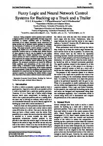
Figure 6 shows the output from a typical discriminator for both tests: on the left is the response from the 2*2 test, on the right the response from the 4*4 test. The figures show the response of the discriminator at various positions within the environment: the lighter the area the higher the response from the discriminator.
4.6 Weightless Networks and the First Eye Attempts to use a standard weightless network with thresholding proved unsuccessful, so the data from the eye were sampled by an array of Minchinton Cells whose outputs were passed to a 150 RAM multi-discriminator network. To quantise an environment to one of n positions, n discriminators were used, with each discriminator being taught to respond strongly to the light patterns characteristic of a particular position within a 4x2m section of the laboratory. First experiments used sixteen discriminators in a [4x4] array, spaced at 0.5m intervals along the x-axis and lm intervals along the y-axis. To achieve rotational invariance, each discriminator could be taught at five rotations of 72o around this point (see figure 5).
Figure 6. Output from one discriminator for each test For the 2*2 test, the discriminator is that for the top left position; the response from the eye is at a maximum when the eye is in that position, and as the eye moves away from that position, the response decreases. For the 4*4 test, the discriminator is that for a position near the middle. Again, the response is highest when the eye is at that position and it falls off monotonically as the eye moves from the trained position. Similar responses are found for the discriminators trained at the other positions.
4.8 The Second Eye
Figure 5. Discriminator positions A tuple size of nine was selected to give a sharp discriminator response. Each discriminator was trained with eleven sets of data collected at random intervals throughout a week. No attempt was made to normalise laboratory lighting, window blind positions or other activity in the laboratory. This process was then repeated using the same data, but this time training four discriminators in a [2x2] regular array, spaced at lm intervals along the x-axis and 2m intervals along the y-axis.
4.7 Results
In the results described above rotation of the insect was ignored. When, however, the insect was rotated, the performance of the system was worse than was expected. This was due to mismatches in the LDRs used, giving rise to large variations in output for a given incident light level. This meant that the RAM neurons had too many different tuples taught - the neurons saturated, which meant that the neurons ‘recognised’ too many input patterns, so there was insufficient discrimination between the positions in the room. It was also felt that 15 elements were insufficient. Therefore a second generation eye has been produced. This has 32 phototransistors, mounted on the faces of half ‘buckie balls’, with the associated electronics mounted inside the ball. The phototransistors are well matched, so they should provide better performance when the insect is rotated, and have a greater resolution. This circuitry processing the signals from the phototransistors contains two sets of multiplexors and a comparator replacing the ADC, thereby incorporating the Minchinton cell processors. Using the comparators rather than an ADC eliminates quantisation noise. It also reduces the mains supply frequency noise which could otherwise cause fluctuations in the data with increased response time of the phototransistors. A block diagram of an eye and associated circuitry is shown in figure 7.
6. Discussion This paper has discussed some of the work done in the Cybernetics Department on its simple mobile robots, in particular the research using neural networks. First a Hopfield-type network, which is used to allow the robot to ‘learn’ how to move around its environment avoiding obstacles. Next a compound eye is described with its neural network processing circuitry. Finally, a technique is outlined, based on an algorithm used in Neural Networks, for combining both networks to allow the robot to navigate back to a position it recognises within its environment. Figure 6. Circuitry of the second eye The eyes were mounted on the robot and the Z80 on the insect was configured with a single discriminator weightless network. The insect was then taught one position in the room and then the response of the network found when the robot was in other positions. The results produced are consistent with the responses shown in figure 6, but they also successfully cope with rotation of the insect.
5. Navigation The output from the eye network gives both an indication of the approximate position of the room and an indication of the direction the robot must travel in order to reach a given position. In addition the ultrasonic sensors provide information which allows the robot to avoid obstacles. The next stage in the work to be described is how all this information is used to allow the robot to travel to a given position whilst avoiding any obstacle in its way. This is to be achieved using an algorithm inspired by the klinotaxic behaviour used by insects to navigate10. This behaviour inspired the Chemotaxis algorithm11: the basic idea of which is also used as an alternative to back propagation in multi-layer perceptron neural networks. A key point in the results of the eye is that the output of the network decreases monotonically as the insect moves from the taught position. The idea for navigation is as follows. The robot is set to move in a random direction, and it continues to move in that direction until it determines that it is moving away from its desired destination. This it can decide using the compound eye: if the response from the discriminator trained on the desired position decreases, the insect is going in the wrong direction. At such a time, the insect chooses another direction randomly, and repeats the process. Eventually the robot reaches the desired position. However, an obstacle may be in the way. Therefore, a priority system is employed: if there are no obstacles visible to the robot, the ‘chemotaxis’ technique is used, but if there are obstacles, obstacle avoidance using the ultrasonic sensors is used to determine how the robot should move. So far, this technique has been established in simulation only, though the learning rules and the compound eye have been successfully employed on the real robots.
References 1.
R.J.Mitchell, D.A.Keating and C.Kambhampati, Learning System for a Simple Robot Insect, Proc. Control '94, pp: 492-497, 1995 2. K. Narendra and M.A.L. Thathachar, Learning Automata: an introduction, PrenticeHall, 1989. 3. J.J.Hopfield, Neural Networks and physical systems with emergent collective properties. Proc. Nat.Acad.Sci., USA 79. 2554-8, 1992 4. D.E.Hebb, The Organisation of Behavour, Wiley, 1949. 5. R.J.Mitchell, D.A.Keating and C.Kambhampati, Neural Network Controller for Mobile Robot Insect, Proc. EURISCON '94, pp: 78-85, 1994. 6. I.Aleksander and T.J.Stonham, Guide to pattern recognition using random-access memories, IEE proceedings pt E, 2, 1, pp29-40, 1979. 7. I.Aleksander and M.J.D Wilson, Adaptive windows for image processing, IEE proceedings pt E, 132, 5, pp233-245, 1985. 8. J.M.Bishop, P.R.Minchinton & R.J.Mitchell, Real Time Invariant Grey Level Image Processing Using Digital Neural Networks, Proc IMechE Conf. EuroTech Direct '91, pp: 187-199, 1991. 9. R.J.Mitchell, J.M.Bishop, S.K.Box and J.F.Hawker, Comparison of methods for processing ‘grey’ level data in weightless networks, Proc Weightless Neural Network Workshop 1995, pp76-81, Univ. of Kent, 1995. 10. P.J.Gullan and P.S.Cranston, The Insects: An Ouline of Entomology, Chapman and Hall, 1994. 11. H.J.Bremermann and R.W.Anderson, An alternative to Back-Propagation: a simple rule for synaptic modification for neural net training and memory, Internal Report, Dept of Maths, Uni of California, Berkeley, 1989.