Neural network and regression based processor load ... - IEEE Xplore

Proceedings of 14th International Conference on Computer and Information Technology (ICCIT 2011) 22-24 December, 2011, Dhaka, Bangladesh

Neural Network and Regression Based Processor Load Prediction for Efficient Scaling of Grid and Cloud Resources Md. Toukir Imamt, Sheikh Faisal Miskhatt, Rashedur M Rahmant, M. Ashraful Amin�

Uepartment of Electrical Engineering and Computer Science, North South University, Bashundhara, Dhaka, Bangladesh. �School of Engineering and Computer Science, Independent University, Bangladesh, Bashundahara, Dhaka, Bangladesh. [email protected],[email protected], [email protected], [email protected] Abstract

An effective and efficient resource allocation policy could benefit the cloud environment by saving cost. To support the continuous load increase, the cloud plaiform needs to create new virtual machines. However, substantial amount of time is required for the creation and the setup of a virtual machine. Therefore, allocating resources in advance based on prediction models could improve the quality of the service of the cloud plaiform. In this paper we present time delay neural network and regression methods for predicting jitture workload in the Grid or Cloud plaiform. We use real world workload traces to test the performance of our algorithms. We also present an overall evaluation of this approach and its potential benefits for enabling efficient auto-scaling of Cloud user resources. Keywo rd s :Cloud Computing, Grid Computing, workload prediction,

neural

network,

time

delay

neural

network,

polynomial regression.

I.

INTRODUCTION

With the emergence of the cloud computing, the need and importance of dynamic resource allocation came into play. Unlike in the classical grid platform, virtual resources can be added or removed from the cloud platform at any time. This property makes the cloud platform more flexible and cost efficient. This dynamic resource allocation could be done from both the cloud client or cloud provider level. The dynamic resource allocation policy makes the cloud platform more attractive. With large companies like Google and Amazon using cloud for large-scale computations, the potential of cloud computing is only starting to unveil. An efficient allocation of resource could mean saving cost for the cloud client. Thus, a provider with an auto­ scaling strategy is more attractive to the client. However, allocating new resources takes up a significant amount of time that is not negligible. Stalling the decision to add new resources till the last moment can significantly deteriorate client experience [5]. On the other hand, for clouds running applications which delivers real time output, this problem is usually solved by gross over allocation [6].This, however, brings us back to static allocation and we lose the primary advantage of cloud platforms. An elegant solution to this problem is allocating resources beforehand based on a prediction model. This will eliminate the performance deterioration of lazy

allocation and if the prediction model is accurate enough, this would not result in significant resource over allocation. Using past workload history to build prediction models for cloud or grid platform is nothing new (e.g. [1], [3], [6] and [5]).Besides auto scaling of resources, these models are useful for synthetic workload generation which can be used to test different scaling policies. The resource scaling decision, off course does not depend solely on the past usage history, cost of resource allocation, cost of migration of jobs and many other factors contribute to the decision of resource scaling in real life situations. For our current work, however, we only focus on the past resource usage. In this paper, we present time delay neural network method and regression method which use the previous usage pattern to predict the future workload. Because of the unavailability of the cloud traces, we used real world traces from grid computer to test our models. We start with a description of related work and then move on to analyzing the trace and presenting the necessary preprocessing done. Section 5 and 6 provides an overview of time delay neural network and the polynomial regression model respectively. In section 7 the performance of the two models is analyzed. II. RELATED WORK

Extensive work has been done in resource usage prediction. Many of the algorithms proposed are based on statistical models. One such model is described in [1]. The authors proposed a statistic-driven model for data­ intensive workloads. The statistical framework Kernel Canonical Correlation Analysis (KCCA) is used to predict the execution time of MapReduce jobs. An analysis of job arrivals in a production data­ intensive Grid was carried out in [2]. The analysis focused on the heavy-tail behaviour and autocorrelation structures, and the modelling is carried out at three different levels: Grid, Virtual Organization(VO), and region. A set of m-state Markov Modulated Poisson Processes (MMPP) is investigated. The experiment showed that MMPPs with a certain number of states were successful in simulating the job traffic at different levels. Although MMPPs were not able to match the autocorrelations for certain vas, in which strong deterministic semi-periodic patterns were observed. In [3] real-world Web access logs collected from popular South Korean blog hosting service Tistory over

987-161284-908-9/11/$26.00 � 2011 IEEE

12 consecutive days was used to investigate user activities of blog servers and the behaviour of user­ created content and their article distribution. The analysis of the LPC cluster usage (Clermont­ Ferrand, France) in the EGEE Grid environment was carried out in [4]. Focusing on the group based activities an infinite Markov based prediction model was proposed with some numerical fitting in between the logs and the model. A very realistic behaviour is observed during simulation which even included bursts. Massively Multiplayer Online Games (MMOG) are a type of client-server applications where strict real-time Quality of Service (QoS) is required. This demand is currently met by over provisioning a large amount of resources, which makes the overall utilization of resources very poor. To address this inefficiency, the authors in [6] described a new prediction-based method for dynamic resource provisioning and scaling of MMOGs in distributed Grid environments. Two different types of neural network were proposed as the prediction model: Feed-foreword network, and Jordan­ Elman recurrent network. The feed foreword network was found to be most accurate, reducing the average over-allocation from 250% (in case of static over­ provisioning) to 25%. Caron et al. [5] used a modified version of Knuth­ Morris-Pratt (KMP) string matching algorithm to match the recent load against previous loads to predict the future workload. The authors proposed an auto-scaling module for the cloud environment and used real-world traces from the Grid computers to test their algorithm. In the experiment with different data length and pattern length combination, the median error is found to be between .9% and 4.08%. A description and comparison of three different auto­ scaling algorithms is given in [8]: auto-Regression of order1 (AR1), Linear Regression, and the Rightscale algorithm. These three algorithms were put side-by-side and compared by a metric proposed in the same article. III. DATASET DESCRIPTION

To evaluate our algorithms we used workload trace from the Large Hadron Collider Computing Grid (LCG). LCG is the grid established to analyse the 15 petabyte of data annually produced by the Large Hadron Collider in CERN (European Organization for Nuclear Research). It is a worldwide collaboration linking thousands of computers, data centres and storage systems. It provides nearly eight thousand scientists real time access to LHC data and the computing facility to analyse this [10]. The trace ranges eleven days of activity. The users submit either serial or parallel jobs and the resource broker finds suitable machines to carry out the processes. The trace is obtained after the jobs are divided into processes; as a result it is impossible to say which processes are part of the same job [9]. A brief description of the trace is given in Table I. For our model, the job arrival time and the running time of the jobs are more important. Though other prediction models [4] are build using user and group information,

we did not make use of this information. Fig. 1 shows the number of jobs arrived daily. Table I summary of LCG trace [9] Nov Date first entry Sun 20 01:00:05 2005 53y 179d 7h 26m CPU time consumed by jobs 46s Number of CPUs in the trace 24,115 Number of jobs in the trace 188041 Number of users in the trace 216 28 Number of groups in the trace 25000 20000 '"

.c

.g ...

0

..

15000 10000 5000 0

11,1,1,1,1,1,1,1,1,1,1, 1

2

3

4

5

6

Days

7

8

9

10

11

Fig. 1 Daily job arrival of the LCG Grid IV. PRE-PROCESSING

For our purpose, we used the job arrival time and the runtime of the job to calculate the workload. The trace is divided into 100 second discrete intervals and for each second the numbers of processors running in parallel is counted. Over the 100 second interval the maximum number of running processor is counted. This way the eleven days of data is divided into 8900 slots. A useful resource pre-allocator must allocate the maximum resource load, which is why we tried to predict the maximum load. We consider this number as the workload of that interval and for the rest of the paper we refer this simply as workload. In our model we used historical data to predict the workload of the next 100 second interval. The pre-processed data of the entire 11 days is shown in Fig. 2. Here, the x-axis denotes the time slots and y­ axis the workload. 4000 3500 "0

.. 0

:ii

(; �

3000 2500 2000 1500 1000 500 0 rl���� rl��M� rl�mM� rl� No:::tr-m --. NqI..OO)rlqI..OOOrl(Y')I..O OO LJ)0U10!..Oril..Ori ...... NI"'- NCX)("(')CX)("(') rlrlNN("(')("(')QQI.l)U1I..OI..O.......... OO

Time(in discrete slots)

Fig. 2 Workload distribution over the 11 days A summary of the data after pre-processing is given in Table II. Table II Summary 0f the data after pre-processIng Min busy processors 28 3693 Max number of busy processors 1622 Avg. Number of busy processors

V. ARCHITECTURE AND ALGORITHMS OF THE TIME DELA Y NEURAL NETWORK

Time delay neural network (TDNN) is a special type of neural network specifically designed for analysis of temporal data [11]. This network was first introduced by Lang and Hinton [12] and Waibel et al. [13]. Its application in phoneme recognition showed 98.5% accuracy compared to 93.7% accuracy in Hidden Markov Model [13]. Though the network was first used for isolated phoneme recognition ([13], [14]), it has been since successfully applied in various other applications. In particular, TDNN has been successfully applied in Electroencephalographic signal classification [15]. The Classification result showed 81% accuracy which is higher than the then reported best result of the BCI 2003 dataset. Time delay networks are useful when the output signal, y(n) depends both on the input signal x(n) and the p previous values of x, x(n-l) ,x(n-2) ....,x(n-p). Here, p is called the tapped delay line memory. At any given time n, the input of the network consists of the vector: x(n)

=

[x(n),x(n-l), ... . . ,x(n-p)y

(1)

Where,p is the number of tapped delay line memory. For a network with one hidden layer, the output of a single neuron j in the hidden layer is given by the equation: (2) Yj cp(Lf=o Wj (Ox(n-1) + bj) =

Here cpO is the activation associated to the neuronj, Wj is synaptic weight and bj is the bias. Therefore the output of a TDNN with m neurons in the hidden layer is: yen)

=

L�l wjyj(n)

(3)

From (2) and (3), y(n)

=

� (t, wi�

Wi (l)x(n-1)

+

bi

)

+

b,

(4) Equation (4) maps the output vector of the network to the input vector. Fig. 3 shows a generalized time delay network. For simplicity, we omitted the bias levels.

Y(II)

We experimented with different training functions and number of hidden layers. The best performance is achieved with one hidden layer and Levenberg­ Marquardt backpropagation training function. The properties of the network fixed for the rest of the paper is given in Table III. Table III Description of the TDNN used in the experiments Levenberg-Marquardt Training function backpropagation 1 Num of hidden layers layer transfer Log-sigmoid 151 function Output layer transfer Linear function 200 Epochs Error function Mean square error(mse) .00005 Performance goal Learning rate .05 Levenverg-Marquardt The backporpagation algorithm is a variation of Newton's method which minimizes functions that are sums of square of other nonlinear function [7]. The algorithm performs well where the error function is the mean square error. VI. REGRESSION

Regression analysis is used for explaining or modelling the relationship between a single variable Y, called the response variable, and one or more predictor, XI" .Xp. For p I it is a uni-variates regression and for p> I it is called multivariate regression [17]. Prior work has experienced the curse of dimensionality when using regression models for long-term prediction. Local polynomial regression has been shown to be a useful nonparametric technique in various local modelling (e.g. [18], [19]). Our regression models are built using the least square method [21]. We used single predictor for building regression models. Nonlinear system prediction posed a significant challenge for the complex system analyst, since the nonlinear structure tends to be very intricate and non­ uniform ([20], [22]). A general form of the non-linear model is provided in (5). Yi ao + a1xi + a1xt + ... a1xf' + Ei(i 1,2, ... , n) (5) Here, a 'i " 'm' and 'e' are constants and represent successive numeric quantities. Here, 'E' represents the random prediction error in the model. The value of m depends on the degree of freedom of the model to be deduced. In general the matrix form of the equation can be viewed in . (6) =

=

=

'

',

[�n�l ; ,;:n :l:n ::�n [�� 1 [�n�l ·

Y

Fig. 3 Time delay neural network

=

1 x x2

• • •

xm

: �

+

G

(6)

The quantities necessary for error computation in our regression models is given in (7) - (13). In the following,

t yiis the original load of i h interval, y is the predicted load and y is the mean load. Sum of squares due to error, SS E=If=l(Yi - y) Sum of squares due to regression, SSR If=l (y; - y)2 Total Sum of squares,

(7) (8)

=

TSS

=

If=l(Yi - y)2

I

At

Tapped Delay Input

Number of Neurons In the hidden layer

Mean Error(%)

4 4 4 4 6 6 6 6 8 8 8 8 10 10 10 10 12 12

3 5 10 15 3 5 10 15 3 5 10 15 3 5 10 15 3 5

0.983992 1.065791 1.23868 3.83778 0.991156 0.88052 1.137537 5.580576 0.983113 0.854314 1.238477 2.112372 0.906768 0.866489 0.860755 1.069478 0.886517 0.993163

12 12

10 15

1.006461 0.960645

(9)

Finally, Mean Squared Error, MSE = SSE/n Where On' = data size Mean Regression Error, MSR = SSE/p Where 'p' = degree of freedom Root Mean Squared Error, RMSE= -VMSE Mean of Absolute percentage error 1 n_ At- Ft MAPE _ I -l

n t

absolute errors of the test. As expected, with the increasing size of the training set, the error gradually decreases. This is more prominent with the percentage error. Table IV Experimental results of different network structures

(10)

(11)

(12)

l

(13)

Where, 'At' is the original value and Ft is the forecasted value. Spline interpolation is a form of interpolation ([16], [24]) where the interpolant is a special type of piecewise polynomial called a spline. In this case, we used cubic spline interpolation since using lower degree polynomial for each spline helps to improve accuracy over depicted predictions. Using the 100 seconds interval processor workload, we predicted workloads of 60 second splines to validate our analysis. Each spline will hold (14) true.

Sex)

{

So (xo),xo � x � Xl Sl(Xl), �f � X � X2

=

Sn-l(X)'Xn-l

�

X

�

(14)

Xn

Now, for each spline, we have the cubic equation, (15) Si(X) aix3 + bix2 + CiX + di Where, 'a', 'b', 'c' and 'd' are constants. This will enable us to validate the predictions devised by the non­ linear regression model. =

VII.

RESULTS

A. Time Delay Neural Network

First, we carried out a series of experiments with varying network structure. The experiments are done with 50% of the trace as training set and the rest as validation set. The results are shown in Table IV. From the results of these experiments we conclude that the network with 8 tapped delay input and 5 neurons in the hidden layer performs the best. We used this architecture for all subsequent experiments. To evaluate the performance of the model with varying size of training set, we divided the entire data in 10 equal sets (each set representing slightly over one days data). Each time, we increased the training data by one set and carried out the validation over the next set. Table V shows the percentage errors and the mean

For a visual comparison of the real workload and predicted workload, we drew the real and predicted workload on the same graph in Fig. 4. In this test, half of the data is used for training and the other half for testing. Here we see that at the scale of the workload, the prediction and the actual load are almost overlapping and the error is insignificant. Table V Validation error with increasing size of trammg set. Size of Trai ning SET (%)

Size of Validati on SET (%)

ERRORS (%)

Mean absolute Error

0-10 0-20 0-30 0-40 0-50 0-60 0-70 0-80 0-90

10-20 20-30 30-40 40-50 50-60 60-70 70-80 80-90 90-100

2.632006 1.333862 1.26131 0.93175 0.982753 0.961959 0.924286 0.760849 0.685992

34.49899 13.23078 22.76481 18.71956 16.51145 11.90714 19.52546 16.9164 16.71241

The maximum absolute error in Fig. 4 is 163. Therefore, to give an estimation of the efficiency of resource scaling based on our prediction model, we

present a dynamic resource allocation model where we always allocate 200 processors more than what our model predicted. Fig. 5 compares this model with a static one where we take the maximum workload and use that for a static allocation. Comparing the dynamic resource allocation model with the static one, we can see, on average the static model does almost 9 times more over allocation than the dynamic model. Over the eleven days the static model does on average 87.8% over allocation compared to 9.9% for the d namic model. 4000

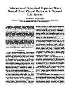
(model 3) F(x) 415.1x8 + 411.8x7 - 2385.4x6 � 5 2074.1x + 4323.8x + 3288.2x3 - 2627.3x2 - Jl21.6x + 1931.8 (18) =

In Fig. 6 the models along with the original workload is shown. Here, in the label "PredictedJ', 'i' is a constant representing the degree of the model. From this graph we can clearly see that, non-linear regression model of degree 8 stands out to be better predictor model than the others. Statistical details of the the model of de ree 8 iv en in Table VI. --Original

3500

4000 "C IV 0 :;;:

3000 "C IV 0 :;;:

0 ==

2500

0 ==

2000 1500

3000

1000

1000 0

500

+------=----11-:--11--

.......... Predicte

d_5

2000

-hI"',.....L----'l,...-=-- -

- - - Predicte d_ 6 -

• •

0

••

••

0

-

...

500000

•

- Predicte

1000000

d_8

Time

Fig. 6 Polynomial Regression Modelling on LCG workload

Time

- - - Predicted Load

-- Actual Load ••••••••••

Table VI Results from Model 3

Absolute Error

Source of variation

Fig. 4 Actual and Predicted workload 5000 4000 "C IV 3000 0 :;;:

e ==

2000 1000

Regression

,---�*}

Error Total

"A�-'" .r

Sum of Squares

Degree of freedom

Mean Error

SSR

P

MSR

3367281312.7

8

12910102.5

SSE

n-p -1

MSE

1588355249.7

8891

178466.8

SST

n-l

4955636562.5

8899 MAPE 23.12% RMSE 433.9359

MAE 341.03

=

0

=

rlm�� mrlm�� mrlm�� mrlm !"oNOO"':- rlf' mO'lLl) Noo...:tOlDmO'l NLI) ..... O('(')LI)OOOmIOOOrlQlCO"I rl .... .... rlrlNNNNC"f')mmmq

Time

-- Actual Load ••••••••••

Dynamic Allocation

- - - Static Allocation

Fig. 5 Dynamic vs. Static resource allocatIOn B. Polynomial Regression Model

The degree of the non-linear model is chosen by successive runs of MATLAB scripts for optimized choice of regression coefficients. To have better analysis and comparisons, we started with a degree greater than or equal to 5 and continued up to degree 12. The best result is achieved by the degree 8 model followed by degree 6 and degree 5 model. For degrees greater than 8 the accuracy of the model sharply declines. Equation (16) (17) and (18) states the corresponding functions for the 5, 6 and 8 degree model respectively.

(model 1) F(x) -78.6x5 2 183.2x - 214. 7x + 1713.1 =

+

51.lx�

(model 2) F(x) -61.2x6 - 78.6x5 3 2 567.4x - 433.6x -214.7x =

+

567.4x3 (16)

+

301.6x�

+

(17)

We validated the developed regression model in (18) by interpolating the processor load predictions. Interpolation on this model means that over intervals of 60 seconds, the model is interpolated to cubic splines. The interpolated results exhibit MAPE value (21.03%) closer the MAPE value of the chosen non-linear model (23.12%). This, in further, validates our decision of choosing the optimal polynomial degree for regression modelling. The deviation of the chosen model and the interpolated results is almost same as that of the deviation of the original trace and the model of degree 8. C. Comparison Between TDNN and Regression Models

A comparison between TDNN and polynomial regression of degree 5, 6 and 8 is given in Table VII. Table VII Comparison between TDNN and Regression Models Model Error (%) MAE 28.8515 1.3226 TDNN 396.7 29.66 Polynomial degree 5 391.7 28.08 Polynomial degree 6 323.8 23.12 Polynomial degree 8

VIII.

[7]

CONCLUSION

Our work shows that time delay neural network performs well in predicting grid workload. We can expect that the model will work equally well when applied to the cloud traces. As we mentioned before, the scaling decision in a cloud platform depends on many factors, however, a predicted workload from a TDNN could be useful for making that decision. The high accuracy necessary for a reliable resource auto-scaling model is achieved by the Time delay network. Our regression model applies moderately to the trace, as evident by spline interpolation. Nevertheless, the analysis depicts of more improvement in regression modelling techniques when dealing with such traces.

M.T.

Hagan,

H.B.

Demuth,

M.H.

Beale,

and

B.

University of Colorado, Neural network design, PWS Boston, MA, 1996. [8]

J.

Kupferman,

J.

Silverman,

P.

into

Browne."Scaling

Jara,

and

the

J.

cloud".

http://cs.ucsb.edu/-jkupferman/docs/ScalingIntoTheClo uds.pdf, 2009. [9]

The Grid Workloads Archive I Homepage. (n.d.). Retrieved July 2, 2011, from http://gwa.ewi.tudelft.nl/

[10]

Worldwide Large Hadron Collider Grid IHomepage (n.d.).

.

Retrieved

July

2,

2011,

from

http://lcg.web.cern.chllcg/public/default.htrn [11]

S.

Haykin,

Neural

Networks:

A

Comprehensive

Foundation, Prentice Hall PTR, 1994. [12]

A. Waibel, T. Hanazawa, G. Hinton, K. Shikano, and KJ.

Lang,

"Phoneme recognition using

neural networks,"

IEEE

time-delay

Transactions on Acoustics,

Speech and Signal Processing, vol. 37, Mar. 1989, pp.

ACKNOWLEDGEMENT

We are thankful to the e-Science Group of HEP at Imperial College, London for graciously providing the the trace. We also thank Hui Li and DrorFeitelson, for making the trace publicly available through the Parallel Workloads Archive. The Grid Workload Archive of the TuDelft University has made the trace available, for this we are thank them. We also thank Shanny Anoep, for providing with an analysis of the trace.

328-339. [13]

KJ. Lang, A.H. Waibel, and G.E. Hinton, "A time-delay neural

network

architecture

for

isolated

word

recognition," Neural Networks, vol. 3, 1990, pp. 23-43. [14]

A. Quiroz, H. Kim, M. Parashar, N. Gnanasambandam, and

N.

Sharma.

Provisioning

for

Towards Enterprise

Autonomic Grids

and

Workload Clouds.

In

Proceedings of the 10 th IEEEIACM International Conference on Grid Computing (Grid 2009), pages 50 57, 2009 [15]

A. Fazel and R. Derakhshani, "A comparative study of time delay neural networks and hidden markov models for electroencephalographic signal classification," Smart

[I]

systems engineering: infra-structure systems engineering,

REFERENCES

bio-informatics

A. Ganapathi, Y. Chen, A. Fox, R. Katz, D. Patterson,

"Statistics-driven workload modelling for the Cloud,"

IEEE

26th

International

Coriference

on

H.

Li,

Muskulus,

M.,Wolters,

L.

"Modeling

Job

Arrivals in a Data-Intensive Grid" .Ed. Frachtenberg, E., Schwiegelshohn,

U.

Job

Scheduling

Strategies

. Vol

Heidelberg,Berlin:Springer.(2007) 4376.DOIIO.10071978-3-540-71035-6_II [3]

X. Kang, H. Zhang, G. Jiang, H. Chen, XiaoqiaoMeng,

Yoshihira, K. , "Measurement, Modelling, and Analysis

of Internet Video Sharing Site Workload: A Case Study,". iEEE International Conference onWeb Services,

2008 (ICWS '08. ) , pp.278-285, 23-26 Sept. 2008.doi: 10.1109I1CWS.2008.28.URL: http://ieeexplore.ieee.orgf

environment." in JSSPP, ser. LNCS, vol. 3834, 2005, pp.

http://www.korf.co.uk/spline.pdf [17]

E. Caron, F. Desprez, and A. Muresan, "Forecasting for Gri and Cloud dComputing On-Demand Resources Based

on

Pattern

International

Matching,"

Conference

on

2010

IEEE

Cloud

Computing

[19]

R. Prodan et aI., "Prediction-based real-time resource provisioning for massively multiplayer online games." Future Generation Computer Systems, Vol. 27, Issue: 7, pp.785-793, 2008.

J.

Fan

and

1.

Gijbels,

"Local

polynomial

fitting,

Smoothing and Regression: Approaches, Computation and Application", 2000, pp. 228-275. [20]

L. Su, "Multivariate Local Polynomial Regression with

!

Application to Shenzhen Component Index," D scret� Dynamics in Nature and Society,Volume 201 I.Hmdawl Publishing,.

[21]

M.E. Crovella and A. Bestavros, "Explaining world wide web traffic self-similarity," Boston University, Boston, MA, 1995.

[22]

Z. Ismail and R. Efendi, "Enrollment Forecasting based on Modified Weight Fuzzy Time Series," Journal of Artificial Intelligence, vol. 4, 2011, pp. 110-118.

[23]

M.E. Crovella and A. Bestavros, "Explaining world wide web traffic self-similarity," Boston University,

456-463. [6]

Fan and 1. Gijbels, "Local polynomial modelling and its

applications", Chapman & HaIl/CRC, 1996.

Second

Technology and Science (CloudCom), IEEE, 2010, pp.

J.J. Faraway, "Practical Regression and ANOVA using R", Citeseer, 2002.

[18]

36-6\. [5]

CJC Kruger, "Constrained Cubic Spline Interpolation for Chemical Engineering Applications." Retrieved from:

670130

E. Medernach, "Workload analysis of a cluster in a grid

and

USA, 2006, p. 311. [16]

stamp/stamp.jsp?tp-&arnumber=4670 I 86&isnumber=4

[4]

biology

2006): held November 6-8, 2006, in St. Louis, Missouri,

for

Parallel Processing. Lecture Notes in Computer Science.

computational

Neural Networks in Engineering Conference (ANNIE

Data

Engineering Workshops (ICDEW 2010), pp.87-92, 2010 [2]

and

evolutionary computation: proceedings of the ArtifiCial

Boston, MA, [24]

C. O'Neill, "Cubic Spline Interpolation" MAE 5093 28

May

2002.

Retrieved

from:

https:llresearch.cc.gatech.edulhumanoids/sites/edu.huma noids/files/cubicspline.odf