Neural Network Architecture Selection: Can function complexity help ? Iv´an G´omez (
[email protected]), Leonardo Franco (
[email protected]) and Jos´e M. J´erez (
[email protected]) Departamento de Lenguajes y Ciencias de la Computaci´ on, Universidad de M´ alaga, Campus de Teatinos S/N, 29071 M´ alaga, Espa˜ na Abstract. This work analyzes the problem of selecting an adequate neural network architecture for a given function, comparing existing approaches and introducing a new one based on the use of the complexity of the function under analysis. Numerical simulations using a large set of Boolean functions are carried out and a comparative analysis of the results is done according to the architectures that the different techniques suggest and based on the generalization ability obtained in each case. The results show that a procedure that utilizes the complexity of the function can help to achieve almost optimal results despite the fact that some variability exists for the generalization ability of similar complexity classes of functions. Keywords: generalization ability, neural network, network architecture, Boolean functions, complexity
1. Introduction Feed-forward neural networks trained by back-propagation have become a standard technique for classification and prediction tasks given their good generalization properties. However, the process of selecting an adequate neural network architecture for a given problem is still a controversial issue. Several theoretical bounds for the number of hidden neurons necessary to implement a given function have been derived using different methods and approximations. Baum and colleagues (Baum and Haussler, 1990) have obtained some bounds on the number of neurons in an architecture related to the number of training examples that can be learnt using networks composed of linear threshold networks. An important contribution about the approximation capabilities of feed-forward networks was made by Barron (Barron, 1994), who computed an estimation of the number of hidden nodes necessary to optimize the approximation error. Camargo et al., (Camargo and Yoneyama, 2001) obtained a result for estimating the number of nodes needed to implement a function using Chebyshev polinomials and using previous results from Scarselli et al. (Scarselli and Tsoi, 1998) about the number of nodes needed for approximating a given function by polynomials. It is worth noting that some of the previous bounds and other existing results have been obtained using the formalism of the Vapnik and Chervonenkis theory, that have helped much to understand the process of generalization in neural networks (Blumer et al., 1989; Haykin, 1994). Singular value decomposition (Wang et al., 2006), geometrical c 2009 Kluwer Academic Publishers. Printed in the Netherlands. °
preprintNEPL.tex; 3/06/2009; 17:15; p.1
2
G´ omez, I. et al.
techniques (Mirchandani and Cao, 1989; Arai, 1993; Zhang et al., 2003), information entropy (Yuan et al., 2003) and the signal-to-noise-ratio (Liu et al., 2007) have been also used to analyze the issue about the optimal number of neurons in a neural architecture. The previous mentioned theoretical results have helped much to understand certain issues regarding the properties of feed-forward neural networks but unfortunately at the time of practical implementations the bounds are loose or difficult to compute. This fact has lead to more practical approaches where researchers investigated the problem of choosing a proper neural architecture through numerical simulations. For example, Lawrence et al. (Lawrence et al., 1996) have shown that the backpropagation algorithm can work relatively well if a large network is chosen and the size of the weights is constrained with regularization techniques such as weight decay (Haykin, 1994). Even if this is the case, still a size has to be chosen and the smaller the architecture the better, specially given the longer training times required for the learning process. Given this situation and to alleviate the computational burden related to the trial-and-error method normally used, different researchers and companies have came out with some rules of thumb, not clearly justified and in some cases based only on their previous experience. In this sense, one of the aims of this work is to analyze differences between different strategies to select the number of neurons in a neural architecture. From the existing research about the influence of the architecture on the generalization ability there is a kind of agreement in the field (Haykin, 1994) that the number of optimal nodes in a neural architecture for obtaining valid generalization depends mainly on three factors: the number of available training samples, the dimension of the function and the complexity of the function. The complexity of the function characterizes how smooth is a given function, and it is clear that the smoother the function the less number of nodes needed and the less number of training samples needed to specify it. The dimensionality of a function might also play an important role given the problem of the curse of dimensionality (See (Haykin, 1994)). It should be also mentioned that there exist alternative approaches for solving the architecture selection problem, like constructive algorithms (Mezard and ˇ Nadal, 1989; Frean, 1990; Weigend et al., 1990; Smieja, 1993) or pruning techniques (LeCun et al., 1990; Haykin, 1994; Liang, 2006). Constructive methods, in general, generate both the architecture and the set of synaptic weights (i.e., the training of the examples is included in the construction process) starting from a small network and adding neurons as the problem requires it. Many different constructive algorithms have been proposed but they have not been extensively applied in practice, and a reason might be that the obtained generalization ability is lower than the obtained with the traditional back-propagation training approach ˇ (Smieja, 1993). Some works have also suggested that large neural networks with small weights trained by back-propagation do not overfit (Lawrence et al., 1996) and thus the use of large architectures where the size of the weights is controlled by some regularization technique, like weight decay or early stopping is an alternative.
preprintNEPL.tex; 3/06/2009; 17:15; p.2
Neural Network Architecture Selection
3
Furthermore, the opposite approach to constructive techniques can also be applied, in this case starting with a large network and after the training process has taken place, a pruning method is applied eliminating less useful weights and neurons (LeCun et al., 1990; Haykin, 1994; Liang, 2006). In this work, by using a recently introduced measure for the complexity of Boolean functions, named generalization complexity (GC measure) (Franco, 2006; Franco and Anthony, 2006), a new method for selecting neural architectures is proposed and compared to some existing rules. The method can be, in principle, only applied to Boolean input data, but we note that through a pre-processing stage real input data can be transformed into binary data and the method applied to them. Extensive numerical simulations with a large set of well known Boolean functions were carried out, testing different architecture sizes and learning parameters, in order to analyze the role of function complexity regarding the optimal number of hidden neurons in an architecture that leads to the largest generalization ability. The paper is structured as follows: section 2 contains the details of the methods utilized in the present study, followed by the results obtained from the extensive numerical simulations that are presented in section 3, to finally discuss the results in section 4. 2. Methods 2.1. Estimation of architecture size by using the GC measure The new method introduced in this work for choosing a neural architecture is based on the use of a complexity measure for Boolean functions, introduced by Franco and colleagues (Franco and Anthony, 2004; Franco, 2006; Franco and Anthony, 2006) and named generalization complexity (GC). The GC-measure, C[f ], was derived from the evidence that bordering examples play an important role on the generalization ability (Franco and Cannas, 2000; Franco and Cannas, 2001) and can be computed by counting the number of pairs of neighboring examples at Hamming distances 1 and 2 having opposite outputs. The first term of the complexity measure, C1 [f ], has been shown to be related to the average sensitivity of a Boolean function, to the number of examples needed to specify a linearly separable function, and to the query complexity of monotone Boolean functions (Franco and Anthony, 2006). The complexity measure terms can also be linked to Harmonic analysis, proven to be extremely useful in a number of areas such as learning theory and circuit complexity (Linial et al., 1993). The GC-measure is defined as: C[f ] = C1 [f ] + C2 [f ],
(1)
where Ci [f ], i = 1, 2 are the terms taking into account pairs of examples at a Hamming distance one and two. Explicitly, the first term can be written as:
preprintNEPL.tex; 3/06/2009; 17:15; p.3
4
G´ omez, I. et al.
C1 [f ] =
1
N ex X
Nex * Nneigh j=1
X
|f (ej ) − f (el )|
(2)
{l|Hamming(ej ,el )=1}
where the first factor, N * 1N , is a normalization one, counting for the total ex neigh number of pairs considered, Nex is the total number of examples equals to 2N , and Nneigh stands for the number of neighbor examples at a Hamming distance of 1. The second term C2 [f ] is constructed in an analogous way. The value of the complexity measure using Eq. 1 ranges from 0 to 1.5. The procedure followed to apply the GC measure for selecting the number of hidden units consists in adjusting the relationship between the optimal number of hidden neurons in a single layer neural network to the generalization complexity of the function, and then use this fit for predicting the number of units in the architecture according to the value of GC for the function under analysis. Clearly the fit, and thus the proposed method, depend on the set of functions used to construct it, but it has to be said that the aim of the present work is to show that the present approach is feasible and that function complexity can be easily estimated and efficiently used for the task of selecting a neural architecture. 2.2. Some existing rules for selecting the number of hidden units This section describes 4 approaches that are currently used in the field of neural networks to choose an architecture. Some of the methods have a theoretical formulation behind, but others are just justified based on experience. The following notation is used: N is the input dimension of the data, Nh represents the number of hidden neurons in the single hidden layer used in the neural architectures and M is used for the output dimension (taken as 1 for all the problems considered). T is used to indicate the number of available training vectors. The four approaches described below correspond to two widely used software frameworks Weka (Witten and Frank, 2005) and Neuralware (Neuralware, 2001) and for two other methods proposed by two researchers (Masters, 1993; Barron, 1994). 1. Weka (Witten and Frank, 2005) is a popular collection of machine learning algorithms for solving real-world data mining problems. Weka permits to compare the predictive accuracy of different learning algorithms. In the implementation of neural network architectures, Weka estimates by default the architecture size as (N + M )/2. It is not clear the justification for the introduction of this rule that has been also suggested on other works (Piramuthu et al., 1994), based on experimental results, and thus it seems that Weka suggests it based on its simplicity and on previous experience. 2. Neuralware (Neuralware, 2001) is a well known commercial software for the implementation of artificial neural networks. They suggest an architecture with
preprintNEPL.tex; 3/06/2009; 17:15; p.4
Neural Network Architecture Selection
5
Nh = T /(5 ∗ (M + N )) neurons. The rationale behind this rule of thumb is to choose the number of hidden units in a way that there are 5 training examples for each synaptic weight in the architecture. 3. An important contribution about the approximation capabilities of feed-forward networks was made by Barron (Barron, 1994), who pointed out that for some classes of smooth functions a number of nodes equal to Nh ∼ Cf (T /(N log T ))1/2 optimizes the mean integrated squared error. Cf is the first absolute moment of the Fourier magnitude distribution of f but computing it is not straightforward (Barron, 1993) (Barron, 1994). Thus, in this work Cf was taken to be equal to 1 and thus the estimated number of hidden units used was Nh = (T /(N log T ))1/2 . √ 4. Masters (Masters, 1993) have suggested to use Nh = N ∗ M neurons in the hidden layer. This rule comes from results indicating that pyramidal neural structures (in which the number of neurons from layer to layer gets reduced) have shown good generalization ability properties. 2.3. The set of test functions The set of single output Boolean functions used for the numerical simulations corresponds to the different outputs of a set of 9 multi-output functions. We consider the cases of N = 10, 11, 12, 13 input dimensions and for each case the number of single output functions was 59, 70, 97 and 70 respectively. These different numbers of functions arise because the output of the functions considered depends on the size of the input. For example, for the function sum considered with 10 inputs, the possible outputs are the 6 significant bits that can be obtained from adding two numbers of 5 bits length. When this same sum function is analyzed in the case N=11, the number of outputs increases to 7 as this is the number of significant outputs that can be obtained from adding two numbers of length 5 and 6. For the case of N = 13 the number of single output functions that can be obtained is larger than the 70 functions considered but due to computational time restrictions the number of functions analyzed was limited to the same set used for the case of N = 11 containing 70 functions. Six out of the nine functions are arithmetic ones forming part of the set of functions used in microprocessors: the functions sum, product, division, subtraction, shifting and square functions. These functions have been also widely analyzed within the area of threshold circuits (Siu and Roychowdhury, 1994). The other three functions used for the tests are Boolean functions previously used in several works and include the i-or-more-clumps, the comparison function and the majority function (Frean, 1990; Mayoraz, 1991; Franco, 2006). The i-or-more-clumps function is a Boolean function that outputs 1 if there are at least i contiguous bit equals to 1 in the input (Frean, 1990). In table I the set of functions is described, where
preprintNEPL.tex; 3/06/2009; 17:15; p.5
6
G´ omez, I. et al.
the name of the function, a short description, and the number of output functions for the case N = 11 are given. For dimensions N = 10, 12 and 13, the number of single output functions varies a bit with respect to the N = 11 case described in detail in table I as the number of outputs changes with the input dimension. As the input dimension grows, new output bits can be considered for each of the 9 functions indicated in table I (conversely for lower dimensions). 2.4. Simulations We performed numerical simulations over the set of 59, 70, 97 and 70 Boolean functions of 10, 11, 12 and 13 inputs respectively described before and shown in Table I for the case of N = 11. The neural architectures used for the simulations include a single hidden layer with a number of neurons between 2 and 30. The use of a single hidden layer neural network is justified on the basis that these architectures can compute any Boolean function and that also this type of network are a standard choice in the field. For each neural network size and set of parameters, a 10-fold complete cross validation scheme was used with the whole set of examples that for the case of Boolean functions comprises 2N examples. Each 10-fold cross validation was set up choosing iteratively a test fold, then a random validation fold, and the remaining eight folds were used for training. The cross validation process was repeated 10 times with a different random seed value. Extreme error values (the minimum and maximum error estimates) were excluded in the computation of the mean generalization ability to reduce the influence of the appearance of local minima in the learning process (V´azquez et al., 2001). In order to avoid overfitting, an early stopping procedure was implemented, in which the generalization error is monitored on the validation set, and the generalization value on a different test set is measured at the minimum of the validation error. The simulations were run on Matlab code under the Linux operating system on a cluster of 25 Pentium IV 2.0 Ghz PCs interconnected through Openmosix. The learning algorithm used was the scaled conjugate gradient back propagation algorithm (Moller, 1993), that combines the model-trust region approach (used in the Levenberg-Marquardt algorithm) with the conjugated gradient approach. This algorithm have shown superlinear convergence properties on most problems and works well with the early stopping procedure applied to avoid overfitting. A brief description of the parameters and their values used for the simulations carried out using the neural network toolbox in Matlab (Demuth and Beale, 1994) are given below: − Starting learning rate: 0.001. Regulate the size of the synaptic weights change (the rate is later adjusted automatically during the training process). − Maximum number of epochs for training: 5000. Stop the training after this maximum number of iterations.
preprintNEPL.tex; 3/06/2009; 17:15; p.6
Neural Network Architecture Selection
7
− Minimum performance gradient: 1e − 6. Stop the training if the magnitude of the gradient drops below this value. − Maximum validation failures: 500. Parameter related to the early stopping procedure. − Sigma parameter: 5.0e−5. Determines the change in weight for the calculation of the approximate Hessian matrix in the scaled conjugate gradient algorithm. − Lambda: 5.0e − 7. Parameter for regulating the indefiniteness of the Hessian. − Neuron transfer function: sigmoid. − Weight values initialization: randomly inside the range [0, 0.25] 2.5. Statistical procedures In order to compare the results obtained from the different rules analyzed in this work, we have applied a series of statistical tests that were used to measure the statistical significance of the differences observed. We have reported in this work differences in performances only when they were statistically significant. The measure used to evaluate the performance of a neural network architecture for a given function was the classification accuracy, computed for the test set by averaging the results over different initial conditions. The classification accuracy is just the number of correctly classified examples divided by the total number of examples. In order to evaluate more precisely the performance of the different neural networks architectures used for each function, Demsar (Demˇsar, 2006) proposes to use the Friedman test (Friedman, 1937) on the averaged results when ten-fold cross-validation is used as sampling method. The Friedman test is a nonparametric test (similar to ANOVA parametric test) that compares the average ranks of K algorithms (K > 2). Under the null hypothesis, the Friedman test states that all the K algorithms perform equivalent and the observed difference is merely random. A p-value of 0.001 was used to consider that the results obtained with a given architecture were better than those obtained with a different one. This relatively low p-value was used in order to minimize the probability of selecting the architectures by purely random fluctuations, and lower p-values were not chosen in order to allow for changes in the size of the neural architectures tested. If the null-hypothesis is rejected (means are significantly different from each other), the Dunn-Sidak posthoc test (H´ajek et al., 1999) is used to study exactly which means differ from each other. This statistical procedure for multiple comparisons provides an upper bound on the probability that any comparison will be incorrectly found significant. Friedman and Dunn-Sidak tests provide the neural network architecture that produces best generalization accuracy for each function. When several architectures with the
preprintNEPL.tex; 3/06/2009; 17:15; p.7
8
G´ omez, I. et al.
same generalization accuracy are selected, the criterium of Occam’s razor is applied to choose the network with the smallest number of neurons. For the comparison of results between two different methods, the Wilcoxon signed rank test for zero median was used (Wilcoxon, 1945).
3. Results The procedure to apply the GC-based method to estimate the optimal neural network architecture for a particular function consists first in finding a fit between the adequate architecture size and the GC of a set of test functions. Once the fit has been obtained for a given dimension, then it is only needed to compute the GC of a new function to obtain the estimated number of neurons in the hidden layer from the fitted curve. In our case, the test set were the 70 functions indicated in Table I for the case N = 11 and 59, 97 and 70 functions for dimensions 10, 12 and 13 respectively. This initial process led us to obtain the optimal neural network architecture for each function (table II, column 3) after exploring sizes from 2 to 30 hidden units, and testing statistical significance in difference on generalization accuracy by using the Friedman test on the results from the ten-fold cross-validation procedure. A two-way analysis was applied as follows: the model that produced the best mean generalization ability for each function fi was selected as the control model, and then, after applying the multiple comparison procedure, the simplest model (in number of hidden neurons) that was not significantly different from the control model was selected. For example, in the case of the function with GC = 0.599 shown in table II, the best performance (averaged over the ten-fold cross-validation procedure) was obtained by the model with 17 hidden neurons (control group), and the Friedman test indicated (p-value < 0.001) that there was statistically significant difference in generalization accuracy across architectures sizes. In this case, the multiple comparison Dunn-Sidak post-hoc test indicated (at the 0.05 significance level) that the generalization ability for the architecture with 10 hidden neurons was not statistically different from the control group, and then the value Nh = 10 is reported in the table. In Figure 1 the results obtained are shown where the optimal architecture size is depicted vs. the GC values for the whole set of 70 functions (the values shown in the figure correspond to columns 1 and 2 in table II). Figure 1 shows how the GC measure is correlated with the number of hidden neurons in the best architectures found and does not indicate whether using the GC measure fit is close to optimality or not because what it is important is the generalization ability obtained from the selected architectures, fact that is analyzed below. The figure shows the individual values and also the best fit obtained by using an exponential function with its corresponding confidence intervals. The exponential function leaded to the best fit in terms of the quadratic error among other functions considered like polynomial or logarithmic ones. The fitting procedure was implemented using the Matlab
preprintNEPL.tex; 3/06/2009; 17:15; p.8
9
Neural Network Architecture Selection
fitting curve procedure and it was not computationally expensive in comparison to the times involved in training the neural networks. For applying the architecture selection process based on the GC measure, a similar fit was used but with only 69 functions instead of the 70, in order to exclude the function under analysis for the architecture selection process. As it is possible to appreciate from the figure, the optimal network size is larger for more complex functions, confirming the fact that the complexity of the function is an important factor in order to select an adequate network size.
35 Best architecture GC fit Confidence interval
Number of hidden neurons
30
25
20
15
10
5
0
0
0.1
0.2
0.3
0.4
0.5
0.6
0.7
0.8
0.9
1
Complexity
Figure 1. Optimal architecture size (number of neurons in the single hidden layer) as a function of the Generalization complexity measure (GC) for 70 Boolean functions of 11 input variables. An exponential fitting curve is also shown with the corresponding confidence intervals.
Thus, to obtain the optimal neural network size using the new method, the value of the GC of the function is computed and the number of units is obtained from the fitted function previously obtained. The results of the method for the 70 functions are shown in columns 4 and 5 in table II, showing both the architecture size estimated by the fitting method and its corresponding generalization accuracy. The results of the other four methods used are also shown in the table in columns 6 to 9. For this four methods, the number of hidden units used are indicated in the second row of the table as they are constant for all functions of the same input dimension.
preprintNEPL.tex; 3/06/2009; 17:15; p.9
10
G´ omez, I. et al.
1 0.95
Generalization ability
0.9 0.85 0.8 0.75 0.7 0.65 Best architecture GC method
0.6
Barron Weka
0.55
Masters Neuralware
0.5
0
0.1
0.2
0.3
0.4
0.5
0.6
0.7
0.8
0.9
1
Complexity
Figure 2. Generalization ability vs function complexity (GC) for 70 Boolean functions. The curves are smoothed fits of the results obtained for the optimum architecture found (”Best architecture”), for the new method introduced (”GC method”) and for 4 other existing rules in the literature (See the text for more details).
The results of all 6 different approaches are shown in Figure 2 showing the generalization ability obtained as a function of the GC measure of the functions. The graphs shown are polynomial fits of the individual values for each of the 70 functions used. The different curves are quite similar for low complexity functions of up to approximately 0.6 (except for the Master rule for which the generalization ability starts to decrease at around 0.4). At this point, the generalization ability of the Barron method and the Weka rule start to go down. The generalization ability remains high for the Neuralware method, for the GC based method and of course for the optimal architectures obtained from exhaustive simulations, but up to around 0.8, where all the curves start to decrease towards 0.5 for functions with a complexity between 0.8 and 1. Note that in the figure, the results of the generalization ability for the Neuralware rule are slightly above the Best architecture ones, fact that in principle cannot be possible but that occurs because we choose the best architecture as the smaller one that shows statistically different results with other size architectures. Thus, the Neuralware curve is not in a statistically significant way above the best architecture curve. A comparison of the performance of the new GC method against the 4 other analyzed rules is shown in Fig. 3. In this figure, the functions with N = 11 were
preprintNEPL.tex; 3/06/2009; 17:15; p.10
Neural Network Architecture Selection
11
grouped according to their GC complexity in 5 groups and the values displayed are for the cases in which the difference in generalization ability was statistical significantly different, measured using a Wilcoxon signed rank test with p < 0.05 (Wilcoxon, 1945). There are less than four bars for each complexity level in the Fig. 3 as the absence of the respective bar indicates that the difference in respect to the use of the GC method was not statistically significant. The largest differences, in which the GC method outperforms the architectures designed using the Masters, Weka and Barron rules, were found in the middle-high and highest complexity groups. The difference between the GC method and the Neuralware approach was also significant, but very small for the lowest, low-middle and middle groups. In the last row of table II, the average values of network size and generalization ability are computed for the introduced GC method and the other rules analyzed. The mean generalization ability was similar for the GC method and the Neuralware (0.938 and 0.939 respectively) showing that the selection of a large architecture can be a good choice independently of the complexity of the function. Nevertheless, the mean neural network size is lower for the GC method, 7.29 neurons vs. the 27 neurons used for the Neuralware rule, and this is a big advantage in the sense of the computational costs involved specially for large dimensional inputs. We have also computed the difference between the new introduced method and the other 4 analyzed rules, comparing the improvement obtained in relationship to the maximum that can be obtained. Figure 4 shows these values for the case of Boolean functions of 11 variables, while in Fig. 5 the cases for N = 10, 12 and 13 are presented. These graphs shows the improvement, I, as a function of the generalization ability obtained from the GC method (Ggc ) over the other 4 methods as a percentage of the optimum (Gopt ), computed using the following equation: I=
Ggc − Gi × 100. Gopt − Gi
For these experiments, the optimal generalization accuracy is computed by an exhaustive search for the best network topology (columns 2 and 3 in table II). Figure 4 shows that, in spite of low values in absolute difference of generalization accuracies, the percentage in improvement exceeds the 50% for several complexity groups of functions, being even up to 100% in some cases, as for the middle groups in dimension 10, 11 and 13, where the GC based method achieved the same level of accuracy than the optimum. An important issue when analyzing the behavior of the generalization ability is how it scales with the dimension of the problem (number of input variables). Thus, we carried out similar simulations for dimensions 10, 12 and 13. The results are shown in Fig. 5 for the percentages in generalization accuracy improvement of the proposed method over the four other rules, computed in a similar way to the results shown in Fig. 4. In these cases, similar results were obtained showing that the GC method can lead to a consistent improvement of the generalization
preprintNEPL.tex; 3/06/2009; 17:15; p.11
12
G´ omez, I. et al.
ability for different input dimensions. We also computed the average size of the architectures generated by the GC method for N = 10, 11 and 12, obtaining a number of neurons equal to 7.17, 7.64, 8.53 and 9.73 respectively. These values were obtained using the same set of 57 functions common to all 3 sets of functions analyzed. We note that our analysis was based on 59, 70, 97 and 70 Boolean functions for dimensions N = 10, 11, 12 and 13 and these numbers represent only a small fraction of the total number of existing functions. Nevertheless, previous results on lower dimensions, where exhaustive simulations were carried out (Franco, 2006) (Franco and Anthony, 2006), indicate that the relationship between the GC complexity and the generalization ability obtained is on average quite accurate for almost all functions. Also we note that our results were obtained in a leave-oneout procedure, in which the function under analysis is not consider for the fitting procedure involved in the estimation of the number of neurons when the GC method is considered and thus, this fact lead us to conjecture that the procedure should work similarly with a different set of functions. We also note that in the reported results obtained using the Barron’s method, we applied a simplified version of the original Barron’s equation with a value of Cf equals to 1. As this value leads to small neural architectures, in general poor generalization values were obtained and thus we have also analyzed the case of using a value of Cf equals to 2. For all the set of functions included in table II (N = 11 and Nh = 8), the average generalization ability obtained was 0.9285, much closer to the results obtained with other methods. We have also compared the computational times involved in the computation of the GC-measure and for the training of the neural architectures, obtaining that both times scale almost exponentially with the number of inputs (or similarly, scale linearly with the number of training examples), as it can be expected. We have computed the average time needed to compute both mentioned tasks, for functions with a number of inputs between 5 and 14 and neural architectures with a number of neurons between 2 and 20, to obtain that on average training a neural architecture cost 140 times more than computing the value of the GC-measure.
4. Conclusions and discussion We have introduced in this work a new approach that permits to select the number of hidden units in a neural network for a given Boolean function. The method is based on a simple measure for the complexity of the functions named generalization complexity (GC). The extensive simulations presented in this work shows that using the GC method for selecting the number of neurons in a feed-forward neural network leads to very efficient results for the generalization ability obtained, in comparison to other four rules tested, and quite close to the optimal values obtained from exhaustive simulations for all possible neural sizes up to 30 neurons. In Figure 2 we showed the average results obtained for all 70 Boolean functions with 11 inputs, and
preprintNEPL.tex; 3/06/2009; 17:15; p.12
Neural Network Architecture Selection
13
it can be clearly seen that the new method leads to results that are quite close to the optimum. Figure 3 shows the difference between the GC method and the other four tested rules for the functions grouped according to their complexity value. For low and middle-low complexity functions the difference is not large, but as the complexity increases the GC method outperformed, in a statistical significant way, 3 out of 4 of the other rules tested. From the 4 different rules analyzed, the Neuralware approach was the closest one to the values obtained by the GC method leading to higher generalization ability values for very complex functions, even if this difference was not statistical significant in comparison to the results obtained from the GC method. The difference of the Neuralware approach against the other three ones studied is that this rule leads to architectures with a larger number of neurons that, combined with the early stopping procedure implemented, worked quite well (this result is in agreement with previous published results about the generalization ability of larger networks (Lawrence et al., 1996)). It is worth noting that as we select the best architectures on statistical basis, given priority to smaller ones, this procedure has the effect that the fitting curve later used for the GC-method is biased towards smaller architectures and this explains the fact that using the Neuralware rule leads in some cases to better results for complex functions when larger architectures are needed. We have also analyzed the difference in generalization ability for different input size functions analyzing the cases for N=10,11,12 and 13 inputs. The obtained results, in terms of the improvement over other alternative rules, were quite similar and show the applicability of the GC method for different input sizes functions (cf. Figs. 4-5). Nevertheless, a limitation of the new GC-method introduced in this work is that it needs a fitting function that has to be obtained in advance for the dimension of the problem to be studied. On the other hand, when the fit is obtained then only the GC measure has to be computed for a new function in order to estimate the neural architecture, procedure that is much faster than training different size neural architectures. We have done some simulation tests to obtain that computing the GC measure is approximately 140 times faster than training a single neural architecture (more details are given at the end of the results section). We hope that from future studies a general fitting curve for different input sizes can be obtained, permitting the application of the GC method to any input size function. We also note that we have used and analyzed for comparison the results obtained using a simplified version of Barron’s formula (Barron, 1993) (Barron, 1994), using a raw approximation for the Fourier coefficients needed, as they are quite difficult to compute. We would like to note that, as Barron’s formula takes into account the effect of the dimension of the problem considered, it could be combined with other approaches, like the based on the GC measure introduced in this work, to obtain an approximation to the number of hidden neurons needed in neural network architectures for higher dimensions to those considered here. It is also worth noting that the present method is restricted to Boolean functions as the generalization complexity measure is only defined for this case. However, real
preprintNEPL.tex; 3/06/2009; 17:15; p.13
14
G´ omez, I. et al.
value input functions can be discretized using standard available methods and thus it is possible to apply the present approach. We are at the moment analyzing this approach and also working on the extension of the GC measure to real input functions.
5. Acknowledgements The authors acknowledge support from CICYT (Spain) through grants TIN200502984 and TIN2008-04985 (including FEDER funds) and from Junta de Andaluc´ıa through grants P06-TIC-01615 and P08-TIC-04026. Leonardo Franco acknowledges support from the Spanish Ministry of Education and Science through a Ram´on y Cajal fellowship. We acknowledge useful discussions with Prof. M. Anthony (LSE, London, UK) and with J.L. Subirats (M´alaga, Spain).
preprintNEPL.tex; 3/06/2009; 17:15; p.14
Neural Network Architecture Selection
15
References Arai, M.: 1993, ‘Bounds on the number of hidden units in binary-valued three-layer neural networks’. Neural Networks 6(6), 855–860. Barron, A. R.: 1993, ‘Universal Approximation Bounds for Superpositions of a Sigmoidal Function’. IEEE Transactions on Information Theory 39(3), 930–945. Barron, A. R.: 1994, ‘Approximation and Estimation Bounds for Artificial Neural Networks’. Mach. Learn. 14(1), 115–133. Baum, E. B. and D. Haussler: 1990, ‘What size net gives valid generalization?’. Neural Comput. 1(1), 151–160. Blumer, A., A. Ehrenfeucht, D. Haussler, and M. K. Warmuth: 1989, ‘Learnability and the VapnikChervonenkis dimension.’. J. ACM 36(4), 929–965. Camargo, L. S. and T. Yoneyama: 2001, ‘Specification of Training Sets and the Number of Hidden Neurons for Multilayer Perceptrons’. Neural Comput. 13(12), 2673–2680. Demuth, H. and M. Beale: 1994, MATLAB Neural Networks Toolbox - User’s Guide Version 4. The Math Works. Demˇsar, J.: 2006, ‘Statistical Comparisons of Classifiers over Multiple Data Sets’. J. Mach. Learn. Res. 7, 1–30. Franco, L.: 2006, ‘Generalization ability of Boolean functions implemented in feedforward neural networks’. Neurocomputing 70, 351–361. Franco, L. and M. Anthony: 2004, ‘On a generalization complexity measure for Boolean functions’. In: Proceedings of the 2004 IEEE International Joint Conference on Neural Networks. pp. 973–978. Franco, L. and M. Anthony: 2006, ‘The influence of oppositely classified examples on the generalization complexity of Boolean functions.’. IEEE Trans Neural Netw 17(3), 578–90. Franco, L. and S. A. Cannas: 2000, ‘Generalization and Selection of Examples in Feedforward Neural Networks’. Neural Computation 12(10), 2405–2426. Franco, L. and S. A. Cannas: 2001, ‘Generalization Properties of Modular Networks: Implementing the Parity Function’. IEEE Trans Neural Netw 12, 1306–1313. Frean, M.: 1990, ‘The upstart algorithm: a method for constructing and training feedforward neural networks’. Neural Comput. 2(2), 198–209. Friedman, M.: 1937, ‘The use of ranks to avoid the assumption of normality implicit in the analysis of variance’. Journal of the American Statistical Association 32, 675–701. ˇ ak, and P. K. Sen: 1999, Theory of rank tests. 2nd ed. Orlando, FL: Academic H´ ajek, J., Z. Sid´ Press. Haykin, S.: 1994, Neural networks: a comprehensive foundation. Prentice Hall. Lawrence, S., C. L. Giles, and A. Tsoi: 1996, ‘What Size Neural Network Gives Optimal Generalization? Convergence Properties of Backpropagation’. Technical Report UMIACS-TR-96-22 and CS-TR-3617, University of Maryland. LeCun, Y., J. Denker, S. Solla, R. E. Howard, and L. D. Jackel: 1990, ‘Optimal Brain Damage’. In: D. S. Touretzky (ed.): Advances in Neural Information Processing Systems II. San Mateo, CA, Morgan Kauffman. Liang, X.: 2006, ‘Removal of hidden neurons in multilayer perceptrons by orthogonal projection and weight crosswise propagation’. Neural Comput. Appl. 16(1), 57–68. Linial, N., Y. Mansour, and N. Nisan: 1993, ‘Constant depth circuits, Fourier transform and learnability’. Journal of the ACM 40, 607–620. Liu, Y., J. A. Starzyk, and Z. Zhu: 2007, ‘Optimizing number of hidden neurons in neural networks’. In: AIAP’07: Proceedings of the 25th conference on Proceedings of the 25th IASTED International Multi-Conference. Anaheim, CA, USA, pp. 121–126, ACTA Press. Masters, T.: 1993, Practical neural network recipes in C++. San Diego, CA, USA: Academic Press Professional, Inc.
preprintNEPL.tex; 3/06/2009; 17:15; p.15
16
G´ omez, I. et al.
Mayoraz, E.: 1991, ‘On the Power of Networks of Majority Functions’. In: IWANN ’91: Proceedings of the International Workshop on Artificial Neural Networks. London, UK, pp. 78–85, SpringerVerlag. Mezard, M. and J.-P. Nadal: 1989, ‘Learning in feedforward layered networks: the tiling algorithm’. Journal of Physics A: Mathematical and General 22(12), 2191–2203. Mirchandani, G. and W. Cao: May 1989, ‘On hidden nodes for neural nets’. Circuits and Systems, IEEE Transactions on 36(5), 661–664. Moller, M. F.: 1993, ‘Scaled Conjugate Gradient Algorithm for Fast Supervised Learning’. Neural Networks 6(4), 525–533. Neuralware, I.: 2001, ‘The reference guide’. http://www.neuralware.com. Piramuthu, S., M. Shaw, and J. Gentry: 1994, ‘A classification approach using multi-layered neural networks’. Decision Support Systems 11, 509–525. Scarselli, F. and A. C. Tsoi: 1998, ‘Universal approximation using feedforward neural networks: a survey of some existing methods, and some new results’. Neural Netw. 11(1), 15–37. Siu, K.-Y. and V. P. Roychowdhury: 1994, ‘On Optimal Depth Threshold Circuits for Multiplication and Related Problems’. SIAM J. Discret. Math. 7(2), 284–292. V´ azquez, E. G., A. Yanez, P. Galindo, and J. Pizarro: 2001, ‘Repeated Measures Multiple Comparison Procedures Applied to Model Selection in Neural Networks’. In: IWANN ’01: Proceedings of the 6th International Work-Conference on Artificial and Natural Neural Networks. London, UK, pp. 88–95, Springer-Verlag. ˇ Smieja, F. J.: 1993, ‘Neural network constructive algorithms: trading generalization for learning efficiency?’. Circuits Syst. Signal Process. 12(2), 331–374. Wang, J., Z. Yi, J. M. Zurada, B.-L. Lu, and H. Yin (eds.): 2006, ‘Advances in Neural Networks - ISNN 2006, Third International Symposium on Neural Networks, Chengdu, China, May 28 June 1, 2006, Proceedings, Part I’, Vol. 3971 of Lecture Notes in Computer Science. Springer. Weigend, A. S., D. E. Rumelhart, and B. A. Huberman: 1990, ‘Generalization by WeightElimination with Application to Forecasting.’. In: NIPS. pp. 875–882. Wilcoxon, F.: 1945, ‘Individual comparisons by ranking methods’. Biometrics 1, 80–83. Witten, I. H. and E. Frank: 2005, Data Mining: Practical Machine Learning Tools and Techniques. Morgan Kaufmann. Yuan, H. C., F. L. Xiong, and X. Y. Huai: 2003, ‘A method for estimating the number of hidden neurons in feed-forward neural networks based on information entropy’. Computers and Electronics in Agriculture 40, 57–64. Zhang, Z., X. Ma, and Y. Yang: 2003, ‘Bounds on the number of hidden neurons in three-layer binary neural networks’. Neural Networks 16(7), 995–1002. Table I. Description of the 70 Boolean functions of N = 11 inputs used for the analysis of different strategies to select the number of hidden units in a feed-forward neural network. id. 1-10 11-17 18-28 29-33 34-39 40-48 49-68 69 70
Function description i-or-more clumps. The output of function i is 1 if there are i contiguous input bits ON. The 7 output bits are the result of the sum of two input numbers of length 6 and 5. The 11 output bits are the result of the product of two numbers of length 6 and 5. The 5 output bits are the result of the quotient between two input numbers of length 6 and 5. The 5 output bits are the result of subtracting a 5 bits number to a 6 bits ones. The 9 output bits are the result of left-shifting the input number i positions. The 20 output bits are the result of the square of the input number The majority function of the input bits. The comparison function of two input numbers of length 6 and 5.
preprintNEPL.tex; 3/06/2009; 17:15; p.16
Neural Network Architecture Selection
17
Figure 3. Difference in generalization ability between the GC based method and the four analyzed rules for Boolean functions on 11 variables grouped according to their complexity. For each level of complexity only the statistically significant differences are reported (See text for more details).
preprintNEPL.tex; 3/06/2009; 17:15; p.17
18
G´ omez, I. et al.
Complexity level
highest
middle-high
middle
low-middle Barron Weka Masters Neuralware
lowest
0
10
20
30
40
50
60
70
80
90
Improvement in generalization ability (% over maximum) Figure 4. Difference in generalization ability as a percentage of the maximum that can be obtained between the GC based method and the four rules analyzed for N = 11. The absence of a bar in each complexity level for any of the 4 methods used for the comparison indicates that the difference was not statistically significant in that case.
preprintNEPL.tex; 3/06/2009; 17:15; p.18
100
19
Neural Network Architecture Selection
Barron Weka Masters Neuralware
Complexity level
Dimension 10
highest middle-high middle lowmiddle lowest
0
10
20
30
40
50
60
70
80
90
100
90
100
90
100
Improvement in generalization (% over maximum) Complexity level
Dimension 12
highest middle-high middle lowmiddle lowest
0
10
20
30
40
50
60
70
80
Improvement in generalization (% over maximum)
Complexity level
Dimension 13 highest middle-high middle lowmiddle lowest
0
10
20
30
40
50
60
70
80
Improvement in generalization (% over maximum) Figure 5. Difference in generalization ability as a percentage of the maximum that can be obtained between the GC based method and the four rules analyzed for N = 10 (top figure), N = 12 (middle figure) and N = 13 (bottom figure).
preprintNEPL.tex; 3/06/2009; 17:15; p.19
20
G´ omez, I. et al.
Table II. Generalization ability and number of hidden neurons obtained for the whole set of 70 Boolean functions with N = 11 inputs using the new GC method and other 4 existing rules. The column indicated by ”Optimum” includes the best results found in the exhaustive numerical simulations with a number of hidden units from 2 to 30. Average values are shown at the bottom row. Optimum
GC method
Barron
Weka
Masters
Neuralware
Nh = 4
Nh = 5
Nh = 3
Nh = 27
Complexity
Nh
Gen.
Nh
Gen.
0.002 0.005 0.013 0.031 0.043 0.065 0.097 0.132 0.191 0.225 0.234 0.241 0.244 0.248 0.264 0.264 0.273 0.273 0.348 0.349 0.349 0.373 0.386 0.407 0.419 0.436 0.443 0.452 0.491 0.491 0.492 0.494 0.494 0.495 0.503 0.508 0.509 0.539 0.539 0.551 0.562 0.586 0.586 0.599 0.600 0.604 0.607 0.643 0.643 0.700 0.706 0.727 0.734 0.777 0.777 0.798 0.807 0.817 0.818 0.840 0.869 0.871 0.900 0.911 0.912 0.930 0.945 0.956 0.967 0.980
2 24 2 2 2 11 2 8 8 2 2 7 2 7 2 2 2 2 8 2 2 5 2 7 5 4 2 2 8 4 2 7 8 5 6 7 3 4 7 5 5 9 7 10 8 5 12 15 6 5 10 14 14 29 4 16 4 6 14 14 16 15 17 14 17 17 6 8 4 7
1.000 0.999 0.997 0.993 0.999 0.991 0.993 0.990 0.996 0.990 0.997 0.987 0.984 0.985 1.000 0.997 1.000 1.000 0.989 0.989 0.999 0.993 0.987 0.987 0.983 1.000 0.963 1.000 0.989 1.000 1.000 0.983 0.999 0.981 0.983 0.957 0.990 0.993 0.989 0.995 0.992 0.997 0.985 0.976 0.995 0.996 0.980 0.995 0.997 0.996 0.916 0.963 0.993 0.944 0.994 0.978 0.983 0.998 0.983 0.791 0.951 0.864 0.732 0.624 0.818 0.808 0.592 0.577 0.544 0.538
3 3 3 3 3 4 4 4 4 5 5 5 5 5 5 5 5 5 5 5 5 6 6 6 6 6 6 6 7 7 7 7 7 7 7 7 7 7 7 7 7 8 8 8 8 8 8 8 8 9 9 9 9 10 10 10 10 11 11 11 11 11 12 12 12 12 13 13 13 13
1.000 0.999 0.997 0.992 0.998 0.989 0.996 0.986 0.992 0.979 0.982 0.983 0.972 0.972 0.984 0.976 1.000 1.000 0.974 0.990 0.976 0.977 0.983 0.987 0.988 0.999 0.987 1.000 0.989 0.999 1.000 0.983 0.999 0.996 0.973 0.952 1.000 1.000 0.981 1.000 0.995 0.997 0.986 0.974 0.996 0.999 0.957 0.993 1.000 1.000 0.916 0.941 0.989 0.927 1.000 0.962 1.000 1.000 0.978 0.774 0.916 0.849 0.709 0.627 0.724 0.732 0.567 0.583 0.529 0.514
1.000 1.000 1.000 1.000 0.999 0.999 0.999 0.999 0.996 0.996 0.997 0.996 0.991 0.992 0.992 0.992 0.997 0.995 0.999 0.996 0.989 0.986 0.987 0.990 0.996 0.988 0.996 0.991 0.986 0.984 0.979 0.985 0.992 0.984 0.988 0.984 0.989 0.979 0.992 0.973 0.991 0.982 0.996 0.975 0.967 0.983 0.943 0.983 0.982 0.972 0.984 0.959 0.982 0.972 0.961 0.968 0.984 0.984 0.994 0.962 0.979 0.976 0.995 0.966 1.000 1.000 1.000 1.000 1.000 1.000 1.000 1.000 0.972 0.974 0.954 0.975 0.968 0.990 0.996 0.963 0.986 0.976 0.997 0.988 0.993 0.972 0.982 0.973 0.975 0.977 0.987 0.984 0.970 0.965 0.922 0.973 0.983 0.979 0.970 0.975 1.000 0.999 0.987 0.948 0.977 0.979 0.994 0.970 1.000 1.000 1.000 1.000 0.964 0.981 0.964 0.993 1.000 1.000 0.994 0.941 1.000 1.000 1.000 1.000 0.981 0.972 0.928 0.971 0.968 0.991 0.887 0.997 0.981 0.986 0.937 0.986 0.978 0.983 0.953 0.976 0.962 0.956 0.899 0.947 1.000 1.000 0.990 1.000 0.999 1.000 0.973 0.963 0.971 0.974 0.943 0.985 0.995 1.000 0.937 0.991 0.992 0.995 0.931 0.966 0.991 0.993 0.937 0.984 0.986 0.981 0.914 0.984 0.952 0.962 0.881 0.973 0.987 0.992 0.895 0.995 0.996 0.996 0.935 0.984 0.916 0.934 0.896 0.965 0.962 0.984 0.853 0.998 0.992 0.997 0.854 1.000 0.996 1.000 0.942 1.000 0.830 0.862 0.760 0.928 0.875 0.927 0.785 0.961 0.900 0.950 0.750 0.996 0.799 0.842 0.720 0.941 0.997 1.000 0.921 1.000 0.795 0.834 0.688 0.988 0.994 1.000 0.895 1.000 0.995 0.998 0.877 1.000 0.807 0.853 0.678 0.992 0.684 0.703 0.641 0.818 0.699 0.751 0.624 0.975 0.698 0.738 0.644 0.872 0.636 0.640 0.603 0.748 0.610 0.623 0.588 0.585 0.619 0.643 0.576 0.860 0.614 0.640 0.564 0.856 0.590 0.592 0.563 0.549 0.570 0.574 0.563 0.553 preprintNEPL.tex; 3/06/2009; 17:15; 0.536 0.543 0.540 0.527 p.20 0.529 0.536 0.523 0.511
0.516
7.46
0.945
7.40
0.938
0.914
0.9226
0.879
0.939