Neural Network Based Edge Detection for Automated Medical Diagnosis

Neural Network Based Edge Detection for Automated

Medical Diagnosis

Dingran Lu1, Xiao-Hua Yu1, Xiaomin Jin1, Bin Li2,3, Quan Chen2,3, Jianhua Zhu4

Abstract - Edge detection is an important but rather difficult task in image processing and analysis. In this research, artificial neural networks are employed for edge detection based on its adaptive learning and nonlinear mapping properties. Fuzzy sets are introduced during the training phase to improve the generalization ability of neural networks. The application of the proposed neural network approach to the edge detection of medical images for automated bladder cancer diagnosis is also investigated. Successful computer simulation results are obtained.

I. INTRODUCTION Edges in images are the curves that characterize the boundaries (or borders) of objects. Edges contain important information of objects such as shapes and locations, and are often used to distinguish different objects and/or separate them from the background in a scene. In image processing, edge detection can be employed to filter out less relevant information while preserving the basic structural properties of an image. It can significantly reduce the amount of data to be processed in the subsequent steps such as feature extraction, image segmentation, registration, and interpretation. Edge detection has found many applications in pattern recognition, image analysis, and computer vision. Since edges are associated with abrupt intensity changes, edge detection is the process to identify and locate such sharp intensity contrasts (i.e., discontinuities) in an image. It is well known that slow changes correspond to small values of derivatives while fast changes correspond to large values of derivatives. Based on this principle, a two-dimensional spatial filter (also called "the gradient operator") is often employed in conventional edge detection algorithms. This filter is designed to be sensitive to detect the gradient of image intensity while yields no response to non-edge (uniform) regions (i.e., the areas with constant intensity) in the image. A variety of filters (or "masks") have been developed to detect various types of edges. For example, different masks can be composed and optimized to detect edges in horizontal, vertical, or diagonal directions, respectively. Once the mask is constructed, it convolves with the entire image, pixel by pixel, to detect edges. Typical conventional edge detection algorithms include the Sobel detector, the Laplacian of Gaussian (LoG) detector

(also termed "the Marr-Hildreth detector"), as well as Canny detector, etc. ([1]) The limitation of the above traditional algorithms is that multiple threshold values need to be set through a trial-and-error process; and these values can dramatically affect the performance of each algorithm. Recently, artificial neural networks (ANN) have been applied to edge detection. Based on the adaptive learning ability and nonlinear mapping ability, neural networks can be trained to detect edges and can serve as nonlinear filters once they are fully trained. In [2], Terry and Vu investigated the application of multi-layer feedforward neural networks for the edge detection of the LADAR (laser radar) image of a bridge. Multiple neural networks are trained by synthetic edge patterns; each one of them can detect a specific edge pattern (e.g., horizontal, vertical, diagonal, etc.). If desired, one can also combine the outputs from the "group" of neural networks to detect multiple types of edges in images. Li and Wang applied neural networks to detect tile defect in [3]. They divided the 8-bit gray-scale image (with 256 levels) into 8 sub gray-scale bit planes, and designed 8 neural networks to process the image in a parallel form. The output of each neural network is then combined based on the weight of each bit plane to generate the final result. The weights for the 8 bit planes (labeled from 1 to 8) are 1/256, 2/256, 4/256, 8/256, 16/256, 32/256, 64/256, and 128/256. Testing results indicate that the middle to high bit planes contain more edge information than the low bit planes (e.g., bit plane 6 has more influence on the accuracy of edge detection than bit plane 1). In n-bit gray-scale images, intensity levels may range from 0 to 2n. To reduce the number of training patterns required to train a neural network, He [4] and Mehrara [5] suggested a shortcut. They converted gray-scale images to binary images first, and then trained neural networks to detect edges in binary images instead of gray-scale images. Since the intensity levels in binary images only have two discrete values (0 and 1), all the possible edge patterns can be included in the training set and the output of neural network converges very fast. However, choosing the appropriate threshold to binarize gray-scale images requires additional works and may also introduce some errors that can affect the accuracy of edge detection. In this research, a multi-layer feedforward neural network is employed for edge detection of gray-scale images. Unlike the multiple neural network approaches proposed in [2] and [3], only a single neural network is used for edge detection.

No pre-processing on gray-scale images is needed, as opposed to the methods presented in [4] and [5]. Furthermore, fuzzy concepts are introduced during the neural network training phase to improve its generalization ability. The proposed neural network approach is applied to some typical test images (e.g., "Lena" and "cameraman") and satisfactory computer simulation results are obtained. With the recent developments on computational intelligence, the design of computerized medical diagnosis systems has received more and more attention. An automated diagnosis system not only saves man power and reduces cost, but also minimizes human bias in the diagnosis process. One of the most challenging tasks in machine learning, however, is to interpret medical images obtained from clinical tests. In this research, we investigate the application of artificial neural networks for bladder cancer cell image detection. Computer simulation results show that the performance of the proposed neural network detector is very promising. The rest of the paper is organized as follows. In section 2, two of the typical conventional algorithms for edge detection, i.e., the Sobel detector and the Laplacian of Gaussian (LoG) detector, are summarized. The neural network model employed for this research is discussed in section 3. In section 4, computer simulation results are presented. Section 5 concludes the paper and also gives the direction for future works.

∇f =

[ ∂f (x, y) ] ∂x

[ grad x ] = grad y ∂f (x, y) ∂y

(1)

where ∇f represents the gradient at location (x, y) of an image f. The direction of the gradient vector points to the direction of the largest possible intensity change (from low intensity to high intensity) and its magnitude (denoted by Mag(∇f ) ) represents the rate of change in that direction:

Mag(∇f ) = (grad x )2 + (grad y ) 2

(2)

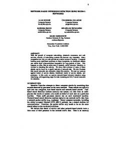
The 3×3, two dimensional Sobel masks for edge detection are shown in Fig. 2 (one for horizontal direction and one for vertical direction). Note that using "2"s in center locations provides image smoothing ([1]). In fact, the edges detected by a Sobel detector are usually several pixels wide due to the smoothing effect. -1 0 1

-2 0 2

-1 -2 -1

-1 0 1

0 0 0

-1 2 1

Fig. 2. The Sobel operator ([1])

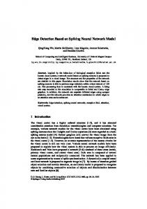
II. THE CONVENTIONAL EDGE DETECTION ALGORITHMS Most of the conventional edge detection algorithms can be classified into two categories, i.e., the gradient based method and the Laplacian based method. The former uses the value of the first order gradient while the latter searches the zero crossings in the second order derivative. The two distinct approaches are illustrated in Fig. 1 ([1]).

Another type of edge detectors finds edges by searching the zero crossings in the second order derivative of the image [1]. The Laplacian of Gaussian (LoG) detector developed by Marr and Hildreth in early '80s (also termed "the MarrHildreth detector") is a typical example. It employs the second order differentiation and searches the points where the Laplacian operator of Gaussian function changes its sign (i.e., crosses zero). The Laplacian operator is defined as:

∇2 f =

∂2 f ∂2 f + ∂x 2 ∂y 2

(3)

The 2-D Gaussian function is defined as:

( x2 + y2 J G(x, y) = exp − 2σ 2

(4)

It can be shown that the expression of the Laplacian of Gaussian (LoG) can be written as ([1]):

∇ G(x, y) = 2

Fig. 1. Conventional edge detection approaches ([1])

Sobel operator (developed in early '70s) is a commonly used discrete first-order gradient detector [1]. The gradient at each pixel in the image is a vector which has two components, one for horizontal direction and the other one for vertical direction:

[ x 2 + y 2 − 2σ 2 ]

σ4

(

x2 + y2 J (5) exp − 2σ 2

One of the major advantages of the Laplacian operator is isotropic - i.e., it is invariant to rotation. This important property indicates that, similar to the characteristics of the human visual system, this filter responds equally to changes in intensity in different directions ([1]). Therefore, unlike the Sobel operator (or other similar first order derivative operators), there is no need to use multiple masks for different directions.

The output of the Laplacian detector is usually a binary image with single pixel thickness lines showing the positions of the zero crossing points. Note the performance of the LoG detector is mainly governed by the standard deviation of the Gaussian function - the higher this value is set, the fewer zero crossings can be detected. III. THE NEURAL NETWORK MODEL In this section, a multi-layer feedforward artificial neural network (ANN) model for edge detection is discussed. It is well known that ANN can learn the input-output mapping of a system through an iterative training and learning process ([6]); thus ANN is an ideal candidate for pattern recognition and data analysis. The ANN model employed in this research has one input layer, one output layer, and one hidden layer. There are 9 neurons in the input layer; in other words, the input of this network is a 9×1 vector which is converted from a 3×3 mask. There are 10 hidden neurons in the hidden layer; and one neuron in the output layer which indicates where an edge is detected. That is, the neural network model is a multi-input, single-output system. The output neuron is linear; the activation function for each hidden neuron is chosen as the hyperbolic function:

f (x) =

1− e − x 1+ e −x

the generalization ability of neural network, fuzzy concepts are introduced during the training phase so that more training patterns can be employed by the neural network. The membership functions are shown in Fig. 4. The grade of membership function, μ (x) , can be defined as:

( (x − ξ ) 2 J μ (x) = exp − 2σ 2 where

(10)

ξ = 1 for "high intensity" and ξ = 0 for "low intensity".

In this research, we choose σ = 0.25.

(a) Edge patterns

(6)

The weights of the neural network are updated using the Levenberg-Marquardt algorithm to minimize the following objective function:

J (k) =

1 2 1 2 e (k) = [d (k) − y(k)] 2 2

(7)

where d is the desired output and y is the output of neural network; e is the output error (i.e., the difference between the neural network output and the desired output); k is the index of a training pair. Let W be the weight matrix of the neural network, then (8) W ( k +1) = W( k ) + ΔW −1

(9) ΔW = ( J a J a + μI ) J a e where J a is the first order derivative of the error function T

(b) Non-edge patterns

Fig. 3. Neural network training patterns

T

with respect to the neural network weight (also called the Jacobian matrix); e is the output error (i.e., the difference between the neural network output and the desired output); μ is a learning parameter. The training patterns for the neural network are shown in Fig. 3. Totally 17 patterns are considered, including 8 patterns for "edge" and 11 patterns for "non-edge". During training, all 17 patterns are randomly selected. For simplicity, all training patterns are binary images. Initial test results show that, though the neural network is fully trained by the above 17 binary patterns, the performance of the neural network detector is poor when it is applied to test images. The reason is that all the test images are gray-scale (i.e., the intensities of images ranging from 0 to 255), not binary. Thus, we normalize the gray-scale intensities so they are within the range between 0 and 1. Furthermore, to improve

1 0.9 0.8 0.7 0.6 0.5 0.4 0.3 0.2 0.1

0

-1

-0.5

0

0.5

1

1.5

2

Fig. 4. Fuzzy membership functions

Now the training patterns in Fig. 3 are represented using fuzzy membership functions. Fig. 5 shows an example of a fuzzy training pattern, where the original pattern (i.e., the first

one in Fig. 3(a)) is shown on the left and the fuzzy pattern is shown on the right: 0 0 0

0 0 0

1 1 1

→

low low low

low low low

high high high

Fig. 5. An example on fuzzy training patterns

Similar to the above example, more training patterns can then be generated using fuzzy concepts to improve the generalization ability of neural network edge detectors. IV. SIMULATION RESULTS In this section, the proposed neural network approach is first tested on two typical test images ("Lena" and "cameraman"), then applied to the cell image for bladder cancer detection. The results obtained by conventional edge detection algorithms, including the Sobel operator and the Laplacian operator are also shown as comparisons. The simulation results on "Lena" and "cameraman" by Sobel, Laplacian, and the neural network detector are shown in Fig. 7 and Fig. 8, respectively. The neural network is trained by a total of 1000 epochs; batch training (batch size = 10) is performed for each training epoch. Similar to the Sobel and Laplacian detector, the trained neural network detector "scans" (but not "convolves") the entire image, pixel by pixel in the size of the 2-D spatial kernel (training pattern), to detect edges. The resulting edge detection images show that the neural network detector not only can detect edges, but also can reveal more details - that in turn provides more information about original images and thus outperforms traditional algorithms.

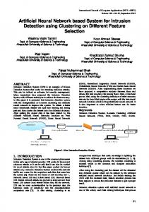
Fig. 6. The bead images under microscope A, B, and C: potential cancer risk; D: no cancer cells found

The proposed neural network detector is also applied to a cell image for bladder cancer detection. Bladder cancer in United States is the fourth most common type of cancer in men and the ninth in women [8]. Early diagnosis is crucial for

cancer prevention, treatment and patient survival. Recently, a new biochemical technique using the special chemical binding property of a specific ligand (called PL4) has developed. In clinical experiments, many small beads are coated with PLZ4 and are mixed with human urine samples. These beads are able to bind to tumor cells, but not to normal cells. Once the binding process is completed, bead images are analyzed under a microscope for further evaluation. Fig. 6 shows four of such images labeled as A, B, C, and D, where the first three images (A, B, and C) show that cancer cells are bounded to the bead, an indication of possible malignant tumor at current; in contrast, image D shows no binding of cancer cells to the bead, indicating no cancer is detected. The current diagnosis is based on a manual cell counting and classification process. Each bead in the image is given a coverage index based on the percentage of coverage of cancer cells on the bead surface; a high coverage index indicates high potential risk of cancer. To automatic this process, edge detection should be performed as the first step for image interpretation. The simulation results of bead images are shown in Fig. 9. These results demonstrate that the neural network detector successfully detects edges in the original image and outperforms the conventional Sobel and Laplacian detectors. V. CONCLUSIONS Edge detection plays an important role in image processing and analysis. In this research, artificial neural networks are successfully applied to detect edges in gray-scale images. Fuzzy sets are introduced during the training phase to improve the generalization ability of neural networks. The real-world application of the proposed approach for bladder cancer detection is also investigated. More tests will be performed in the future to further improve the neural network edge detector.

(a) Original image

(a) Original image

(b) Sobel detector

(b) Sobel detector

(c) Laplacian detector

(c) Laplacian detector

(d) Neural network detector

(d) Neural network detector

Fig. 7. Simulation results on "Lena" image

Fig. 8. Simulation results on "cameraman" image

REFERENCES

(a) Original image

(b) Sobel detector

(c) Laplacian detector

(d) Neural network detector Fig. 9. Simulation results on the cell image for bladder cancer detection

[1] Gonzalez, R., Woods, R., Digital Image Processing, 3rd Edition. Prentice Hall, 2008. [2] Terry, P., Vu, D., "Edge Detection Using Neural Networks", Conference Record of the Twenty-seventh Asilomar Conference on Signals, Systems and Computers. Nov. 1993, pp.391-395. [3] Li, W., Wang, C., Wang, Q., Chen, G., "An Edge Detection Method Based on Optimized BP Neural Network", Proceedings of the International Symposium on Information Science and Engineering, Dec. 2008, pp. 40-44. [4] He, Z., Siyal, M., "Edge Detection with BP Neural Networks", Proceedings of the International Conference on Signal Processing, 1998, pp.1382-1384 [5] Mehrara, H., Zahedinejad, M., Pourmohammad, A., "Novel Edge Detection Using BP Neural Network Based on Threshold Binarization", Proceedings of the Second International Conference on Computer and Electrical Engineering, Dec. 2009, pp. 408-412. [6] Haykin, S., Neural Networks: A Comprehensive Foundation, Prentice Hall, 1999. [7] Neural Network Toolbox User’s Guide, The Mathworks. [8] http://en.wikipedia.org/wiki/Bladder_cancer