Edge Detection Based on Spiking Neural Network

Edge Detection Based on Spiking Neural Network Model QingXiang Wu, Martin McGinnity, Liam Maguire, Ammar Belatreche, and Brendan Glackin School of Computing and Intelligent Systems, University of Ulster at Magee Campus Derry, BT48 7JL, Northern Ireland, UK {q.wu,tm.mcginnity,lp.maguire,a.belatreche,b.glackin}@ulster.ac.uk

Abstract. Inspired by the behaviour of biological receptive fields and the human visual system, a network model based on spiking neurons is proposed to detect edges in a visual image. The structure and the properties of the network are detailed in this paper. Simulation results show that the network based on spiking neurons is able to perform edge detection within a time interval of 100 ms. This processing time is consistent with the human visual system. A firing rate map recorded in the simulation is comparable to Sobel and Canny edge graphics. In addition, the network can separate different edges using synapse plasticity, and the network provides an attention mechanism in which edges in an attention area can be enhanced. Keywords: Edge detection, spiking neural networks, receptive field, attention, visual system.

1 Introduction The visual cortex has a highly ordered structure [1-2], and it has attracted considerable attention from theoretical neurobiologists and computer scientists. For example, various network models for the visual cortex have been simulated using spiking neurons since the Hodgkin and Huxley equations [3] were regarded as a basic spiking neuron model [4]. Retinal ganglion cells convey the visual image from the eye to the brain [1-2]. Neurobiologists have found that various receptive fields exist in the visual cortex [1-2]. However, an accurate representation of the neuron circuits for the visual cortex is still not very clear. Various neural network models have been proposed to explain how the visual system is able to process on image efficiently. Knoblauch and Palm have proposed a network [5-6] consisted of three areas (retina, primary visual cortex, and central visual area). Each area is composed of several neuron populations and reciprocally connected. The network has been applied to scene segmentation by means of spike synchronization. A dynamically coupled neural oscillator network is proposed to segment image in [7]. By means of attention-guided object selection and novelty detection, an oscillatory model is proposed to recognise objects by combining consecutive selection of objects and discrimination between new and familiar objects [8]. D.-S. Huang, L. Heutte, and M. Loog (Eds.): ICIC 2007, LNAI 4682, pp. 26–34, 2007. © Springer-Verlag Berlin Heidelberg 2007

Edge Detection Based on Spiking Neural Network Model

27

A model of self-organizing maps of spiking neurons has been applied in computational modelling of the pattern interaction and orientation maps in the primary visual cortex [9-11]. Spiking neurons with leaky integrator synapses have been used to model image segmentation and binding by synchronization and desynchronization of neuronal group activity. The model, which is called RFSLISSOM, integrates the spiking leaky integrator model with the RF-LISSOM structure, modelling self-organization and functional dynamics of the visual cortex at a more accurate level than earlier models. These neural network models can be applied to explain some of the behaviours of the visual system in the human brain. The spike synchronization network in [5-6] can be applied to explain why the visual system can perform high-level visual processing tasks in a limited time of 100-150 ms. This model is based on a firing order encoding scheme which is called spike wave, in which neurons are allowed to fire only once during a period. The model can explain how this information embedded in the first wave of spikes generated in the retina can be decoded by post-synaptic neurons, and how it can propagate in a feed-forward way through a simple hierarchical model of the visual system, to implement fast and reliable object recognition. Although to date there has been no experimental observation to directly confirm the model, there is also no direct experimental evidence of the contrary. The literature shows that many experimental results tend to favour the hypothesis in the model. Actually, many neuron models and receptive field models have been described in neuroscience [2]. In this paper, different receptive field models [2] are used to construct a spiking neural network which is used to simulate the visual cortex for edge detecting. Firstly, a network model based on integrate-and-fire neurons is detailed in Section 2. The receptive fields of spiking neurons play a crucial role for edge detecting in the network. The behaviours of the neurons with the receptive fields are analyzed in Section 3. Simulation results for edge detecting and comparison with other edge detecting algorithms are shown in Section 4. Discussions about the network are presented in Section 5.

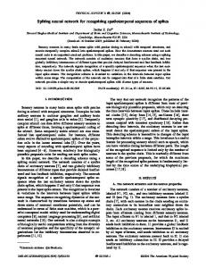
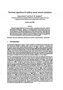
2 Spiking Neural Network Model for Edge Detection The human visual system performs edge detection very efficiently. Neuroscientists have found that there are various receptive fields from simple cells in the striate cortex to those of the retina and lateral geniculate nucleus (see page 236-248 in [2]) and the neurons can be simulated by the Hodgkin and Huxley neuron model. Based on these receptive fields and the neuron model, a network model is proposed to detect edges in a visual image in this paper. The structure of the network is shown in Fig. 1. Suppose that the first layer represents photonic receptors. Each pixel corresponds to a receptor. The intermediate layer is composed of four types of neurons corresponding to four different receptive fields respectively. ‘X’ in the synapse connections represents an excitatory synapse. ‘Δ’ represents an inhibitory synapse. Each neuron in the output layer integrates four corresponding outputs from intermediate neurons. The firing rate map of the output layer forms an edge graphic corresponding to the input image.

28

Q. Wu et al.

x’

x wup

y

wdown RFrcpt

(x,y)

wleft

right

w Receptor layer

' '' ' X' ' ' XX ' XX XX X X XX X 'X X X ' ' X '' '' ' ' ''X ' ' XX ' ' XX ' X X X X XX ' XX ' ' XX ' X' '' '

y’ N1 wN1 N2 wN2

(x’,y’)

N3 wN3 N4

wN4

Intermediate layer

Output layer

Fig. 1. Spiking Neural Network Model for Edge Detecting

There are four parallel arrays of neurons in the intermediate layer each of the same dimension as the Receptor layer. These arrays are flagged as N1, N2, N3 and N4 and only one neuron in each array is shown in Figure 1 for simplicity. Each of these layers perform the processing for up, down, left and right edges respectively and are connected to the receptor layer by differing weight matrices. These weight matrices can be of varying sizes to represent the width of the receptive field under consideration. For example in Figure 1 neuron N1 connects to receptive field RFrcpt in the receptor layer through synapse strength distribution matrix wup, and responds to an up-edge within the field. If a uniform image within RFrcpt makes a uniform output, the outputs through synapses in wup reach neuron N1. Connections through the upper-half of the weight matrix represent inhibitory synapses which depress the membrane potential of Neuron N1 while connections through the lower-half excitatory synapses potentiate the membrane potential of Neuron N1. Therefore the membrane potential of Neuron N1 has not been changed, and no spikes are generated by Neuron N1. However, if an edge image within the RFrcpt is incident on lower-half receptors with a strong signal and the upper-half receptors with a very weak signal, then the strong signal will potentiate (due to the excitatory synapses) neuron N1, but the weak signal will not depress the membrane potential significantly. The membrane potential of Neuron N1 rise up fast and generates spikes frequently to respond to an up-edge within its receptive field. The synapse distribution matrix wup plays a role as a filter for up-edge within the receptive field. By analogy, neuron N2 with synapse strength


29

distribution wdown can best respond to a down-edge within the receptive field; neuron N3 with synapse strength distribution wleft can best respond to a left-edge; and neuron N4 with synapse strength distribution wright can best respond to a right-edge. Neuron (x’, y’) in the output layer integrates the outputs from these four neurons from the neuron arrays in the intermediate layer, and can respond to any direction edge within receptive field RFrcpt. The network model is presented in following sections.

3 Spiking Neuron Model and Receptive Fields Simulation results show that the conductance based integrate-and-fire model is very close to the Hodgkin and Huxley neuron model [11-16]. The conductance based integrate-and-fire model is applied to the aforementioned network model. Let Gx,y represent gray scale at (x,y)∈RFrcpt, q ex x, y represent peak conductance caused by excitatory current from a receptor at (x,y), and qih x, y represent peak conductance caused to inhibitory current from a receptor at (x,y). For simplicity, suppose that each receptor can transform a value of gray scale to peak conductance by the following expressions. qxex, y = α Gx, y ;

qih x , y = β Gx , y

(1)

where α and β are constants. According to the conductance based integrate-and-fire model [15-16], neuron N1 is governed by the following equations.

g xex, y (t ) dt g ih x , y (t ) dt

cm

=−

=−

1

τ ex 1

τ ih

g xex, y (t ) + α Gx , y

(2)

g ih x , y (t ) + β Gx , y

(3)

dvN1 (t ) = gl ( El − vN 1 (t )) + dt ( x , y )∈RF

∑

rcpt

+

∑

( x , y )∈RFrcpt

_ ih ih wup x , y g x , y (t )

Aih

wup _ ex g xex, y (t ) x,y

Aex

( Eex − vN 1 (t ))

(4)

( Eih − vN1 (t ))

ih where g ex x , y (t ) and g x , y (t ) are the conductance for excitatory and inhibitory synapses

respectively, τex and τih are the time constants for excitatory and inhibitory synapses respectively, vN 1 (t ) is the membrane potential of neuron N1, Eex and Eih are the reverse potential for excitatory and inhibitory synapses respectively, cm represents a capacitance of the membrane, gl represents the conductance of membrane, ex is short _ ex for excitatory and ih for inhibitory, wup represents the strength of excitatory x, y _ ih synapses, wup represents the strength of inhibitory synapses, Aex is the membrane x, y

30

Q. Wu et al.

surface area connected to a excitatory synapse, and Aih is the membrane surface area connected to a inhibitory synapse. According to the description of biological receptive _ ex _ ih fields [2], values for wup and wup are expressed as follows. x, y x, y 0 if ( y − yc ) ≤ 0 ⎧ 2 2 _ ex ⎪ ( ) ( ) x x y y − − wup = c c ⎨ x, y − − 2 2 δx δy ⎪ if ( y − yc ) > 0 ⎩ we max e

(5)

if ( y − yc ) > 0 ⎧ 0 ⎪ 2 ( x − xc ) ( y − yc )2 =⎨ − − δx δy ⎪w if ( y − yc ) ≤ 0 ⎩ i max e

(6)

_ ih wup x, y

where (xc, yc) is the centre of receptive field RFrcpt, (x,y)∈RFrcpt, δx and δy are constants, wemax and wimax are the maximal weights for excitatory synapses and inhibitory synapses respectively. By analogy, Neuron N2, N3, and N4 are governed by a set of equations similar to that for neuron N1. When the membrane potential reaches a threshold vth the neuron generates a spike, and then it enters a refractory state. After period τref the neuron can integrate inputs to generate another spike. Let SN1(t) represent a spike train which is generated by neuron N1. ⎧1 S N 1 (t ) = ⎨ ⎩0

if neuron N1 fires at time t. if neuron N1 does not fire at timet.

(7)

By analogy, let SN2(t), SN3(t) and SN4(t) represent spike trains for neurons N2, N3 and N4 respectively. Neuron Nx’,y’ in the output layer is governed by the following equations. g xex', y ' (t ) dt

=−

1

τ ex

g xex' y ' (t ) + ( wN 1S N 1 (t ) + wN 2 S N 2 (t )

(8)

+ wN 3 S N 3 (t ) + wN 4 S N 4 (t )) cm

dvx ', y ' (t ) dt

= gl ( El − vx ', y ' (t )) +

g xex', y ' (t ) Aex

( Eex − vx ', y ' (t ))

(9)

Note that Neuron Nx’,y’ is connected to intermediate neurons only by excitatory synapses. Let Sx’,y’ (t) represent spike a train generated by Neuron Nx’,y’ in output layer. The firing rate for Neuron Nx’,y’ is calculated by the following expression. rx ', y ' =

1 t +T S x ', y ' (t ) T t

∑

(10)

By plotting this firing rate as an image with a colour bar an edge graphic for the input image is obtained.


4

31

Simulation Results

The network model was implemented in Matlab using a set of parameters for the network: vth = -60 mv. vreset = -70 mv. Eex= 0 mv. Eih= -75 mv. El= -70 mv. gl =1.0 μs/mm2. cm=10 nF/mm2. τex=4 ms. τih=10 ms. τref =6 ms. Aih=0.028953 mm2. Aex=0.014103 mm2. These parameters are consistent with biological neurons [3]. Synapse strengths are controlled by wemax and wimax. The proportion between wemax and wimax can be adjusted to ensure that the neuron does not fire in response to a uniform image within its receptive field. Contrasting the maximal weights wemax provided in [15] , wemax is set to 0.7093 for excitatory synapses, and wimax is set to 0.3455 for inhibitory synapses. Image gray scale values are normalized in a real number in the range of 0 to 1. Therefore, α and β are set to 1/max_value_in_image. The size of RFrcpt may be set in the range 2×2 to 6×6. The parameters δx and δy can be applied to control sensitiveness to edges. Experiments for different values of δx , δy and size of RFrcpt have been done. The results show that the larger of δx , δy and size of RFrcpt, the lower is the detector's sensitivity to noise. On the other hand, the larger of δx , δy and size of RFrcpt, the edge become more vague. There is a tradeoff for selection of the values. For the synapse strength distribution matrix wup and wdown, δx should be set to δx > δy to get a horizontal shape that will be consistent with the receptive field in biological system [2]. In the results presented, δx =6, δy=2, and the size of RFrcpt is set to the 5×5. For example, the 5×5 receptive field matrices for wup_ex and wup_ih , which are calculated according to (5) and (6), are shown as follows.

w up_ex

0 0 0 0⎤ ⎡0 ⎡.11 .12 .13 .12 .11⎤ ⎢0 ⎥ ⎢.31 .34 .35 .34 .31⎥ 0 0 0 0⎥ ⎢ ⎢ ⎥ =⎢0 0 0 0 0 ⎥ w up_ih = ⎢ 0 0 0 0 0⎥ ⎢ ⎥ ⎢ ⎥ 0 0 0 0⎥ ⎢.31 .34 .35 .34 .31⎥ ⎢0 ⎢⎣.11 .12 .13 .12 .11⎥⎦ ⎢⎣ 0 0 0 0 0 ⎥⎦

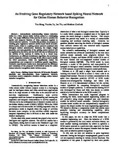
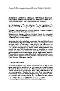
Fig. 2. Screen shot image from AIBO robot control system

32

Q. Wu et al.

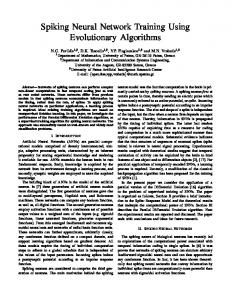
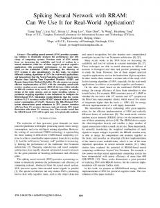
If a screen shot, which is shown in Fig. 2, is presented to the network, the firing rate map on the output layer is obtained as shown in Fig. 3 reflecting the edges for the input image. Bright lines show that the corresponding neurons fires with a high frequency and indicate the edges with high contrast. Dark lines show that the corresponding neurons fires with a low frequency and indicate the edges with low contrast. Using the firing rates, different contrast edges can be separated.

Fig. 3. Firing rate map from output layer

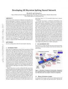
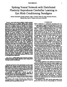
In order to compare with Sobel and Canny edge detection methods, the results for benchmark image Lena photo are shown in Fig. 4.

Lena photo

Sobel edges

Canny edges

Neuron firing rate map

Fig. 4. Comparison of neuron firing rate map with other edge detecting methods

5 Discussion Spiking neural networks are constructed by a hierarchical structure that is composed of spiking neurons with various receptive fields and plasticity synapses. The spiking neuron models provide powerful functionality for integration of inputs and generation


33

of spikes. Synapses are able to perform different computations, filters, adaptation and dynamic properties [17]. Various receptive fields and hierarchical structures of spiking neurons enable a spiking neural network to perform very complicated computations, learning tasks and intelligent behaviours in the human brain. This paper demonstrated how a spiking neural network can detect edges in an image. Although the neuron circuits in the brain for edge detection are not very clear, the proposed network model is a possible solution based on spiking neurons. In the simulation, the neuron firing rate map for edges can be obtained with a time interval 100 ms. This time interval is consistent with the biological visual system. If the model is simulated by Matlab program in a PC with CPU 1.2G, it takes about 50 seconds to get a firingrate map for an image with 500x800 pixels. If the network model is implemented in parallel on hardware, the edge detection can be achieved within 100 ms. Therefore, this model can be applied to artificial intelligent systems. If synaptic plasticity is considered, different scales of firing rate map for edges can be obtained. For example, the human visual system can focus attention on a selected area and enhance resolution and contrast. Based on this model, an attention area can be enhanced by simply strengthening wemax and wimax. Fig. 5 shows that an attention area around point (650,350) is enhanced. Within the attention area, wemax=0.7093 and wimax=0.3455. Outside of the attention area, w’emax= wemax/4 and w’imax= wimax /4.

Fig. 5. Attention area around (650,350)

By adjusting neuron thresholds in the intermediate layer and output layer, the resolution and contrast in the attention area can also be enhanced. This paper has only investigated edge detection based on spiking neurons. Future work will consider different approaches to further improve the network and investigate the use of lateral connections within the intermediate layers or output layer.

34

Q. Wu et al.

References 1. Hosoya, T., Baccus, S.A., Meister, M.: Dynamic Predictive Coding by The Retina. Nature, 436 (2005) 71 - 77 2. Kandel, E.R., Shwartz, J.H.: Principles of Neural Science. Edward Amold (Publishers) Ltd. (1981) 3. Hodgkin, A., Huxley, A.: A Quantitative Description of Membrane Current and Its Application to Conduction and Excitation in Nerve. Journal of Physiology. (London). 117 (1952) 500-544 4. Neuron Software download website: http://neuron.duke.edu/ 5. Knoblauch, A., Palm, G.: Scene Segmentation by Spike Synchronization in Reciprocally Connected Visual Areas. I. Local Effects of Cortical Feedback, Biol Cybern. 87(2002) 151-67 6. Knoblauch, A., Palm, G.: Scene Segmentation by Spike Synchronization in Reciprocally Connected Visual Areas. II. Global Assemblies and Synchronization on Larger Space and Time Scales. Biol Cybern. 87 (2002) 168-84 7. Chen, K., Wang, D.L.: A Dynamically Coupled Neural Oscillator Network for Image Segmentation. Neural Networks. 15(3) (2002) 423-439 8. Purushothaman, G., Patel, S.S., Bedell, H.E., Ogmen, H.: Moving Ahead Through Differential Visual Latency, Nature. 396 (1998) 424-424. 9. Choe, Y., Miikkulainen, R.: Contour Integration and Segmentation in A Self-organizing Map of Spiking Neurons. Biological Cybernetics. 90(2) (2004) 75-88 10. Borisyuk, R.M., Kazanovich, Y.B.: Oscillatory Model of Attention-guided Object Selection and Novelty Detection. Neural Networks. 17(7) (2004) 899-915 11. Koch, C.: Biophysics of Computation: Information Processing in Single Neurons. Oxford University Press. (1999) 12. Dayan, P., Abbott, L.F.: Theoretical Neuroscience: Computational and Mathematical Modeling of Neural Systems. The MIT Press, Cambridge, Massachusetts. (2001) 13. Gerstner, W., Kistler, W.: Spiking Neuron Models: Single Neurons, pulations, Plasticity. Cambridge University Press. (2002) 14. Müller, E.: Simulation of High-Conductance States in Cortical Neural Networks, Masters thesis, University of Heidelberg, HD-KIP-03-22. (2003) 15. Wu, Q.X., McGinnity, T.M., Maguire, L.P., Glackin, B., Belatreche, A.: Learning Mechanism in Networks of spiking Neurons. Studies in Computational Intelligence, Springer-Verlag. 35 (2006) 171–197 16. Wu, Q.X., McGinnity, T.M., Maguire, L.P., Belatreche, A., Glackin, B.: Adaptive CoOrdinate Transformation Based on Spike Timing-Dependent Plasticity Learning Paradigm, LNCS, Springer. 3610 (2005) 420-429 17. Abbott, L.F., Regehr, W.G.: Synaptic Computation. Nature. 431(2004) 796 – 803