construction and selection procedure for neural modeling. We finally ..... In section IV.2.1, we recall the test of fit, which, if repetitions have been performed, allows to discard ..... Discussion. We can now make several statements and comments:.
Published in IEEE Transactions on Neural Networks vol. 14 N°4, pp. 804-819.
NEURAL NETWORK CONSTRUCTION AND SELECTION IN NONLINEAR MODELING Isabelle Rivals and Léon Personnaz Équipe de Statistique Appliquée, École Supérieure de Physique et de Chimie Industrielles, 10, rue Vauquelin - 75231 Paris Cedex 05 - France.
Abstract In this paper, we study how statistical tools which are commonly used independently can advantageously be exploited together in order to improve neural network estimation and selection in nonlinear static modeling. The tools we consider are the analysis of the numerical conditioning of the neural network candidates, statistical hypothesis tests, and cross validation. We present and analyze each of these tools in order to justify at what stage of a construction and selection procedure they can be most useful. On the basis of this analysis, we then propose a novel and systematic construction and selection procedure for neural modeling. We finally illustrate its efficiency through large scale simulations experiments and real world modeling problems. Keywords Growing and pruning procedures, nonlinear regression, neural networks, least squares estimation, linear Taylor expansion, ill-conditioning detection, input selection, model selection, leave-one-out cross validation, statistical hypothesis tests. Nomenclature We distinguish between random variables and their values (or realizations) by using upper- and lowercase letters; all vectors are column vectors, and are denoted by boldface letters; non random matrices are denoted by light lowercase “Courier” letters.
n x
number of inputs non random n-input vector
2
Yp m x W s2 q q f x, q , q ∈ q N x k, ypk k=1 to N
R
J q QLS qLS iN x = x 1 x 2 … xN T f x, q z = z 1 z 2 … zN T pz = z z T z -1 z T R = Yp – f x,QLS r T S2 = R R N–q s2 h e k k=1 to N a p Abbreviations ALOOS LOOS LS LTE MSTE MSPE
random scalar output depending on x mathematical expectation, or regression function, of Yp given x random variable with zero expectation denoting additive noise variance of W number of parameters q-parameter vector family of nonlinear functions of x parameterized by q size of the data set data set of N input-output pairs, where the x k are non random n-vectors, and the ypk are the corresponding realizations of the random outputs Ypk value of the least squares cost function least squares estimator of the parameter vector least squares estimate of the parameter vector (N,N) identity matrix non random (N,n) input matrix N-vector f x 1, q … f x k , q … f x N, q T Jacobian matrix with z k = ∂f x k , q ∂q q = qLS orthogonal projection matrix on the range of z ("hat" matrix) least squares residual random N-vector value of R estimator of s 2 value of S2 Hessian matrix of the cost function J leave-one-out errors (p, q) restriction matrix for the test of the significance of p parameters ratio of the ALOOS to the MSPE
approximate leave-one-out score leave-one-out score least squares linear Taylor expansion mean square training error mean square performance error
3 I. INTRODUCTION The problem of constructing the best neural model given a finite data set is one of the most important and discussed problems. In the literature about nonlinear model estimation and selection, one can find many papers about heuristic and statistical tools and procedures, such as hypothesis testing, information criteria, or cross validation [Leontaritis & Billings 1987] [Efron & Tibshirani 1993] [Moody 1994] [Anders & Korn 1999]. These procedures are sometimes compared one to another [Anders & Korn 1999], but there is seldom an attempt to use these methods together at different stages of a general and systematic procedure. In the same spirit, additive (or constructive, or growing) methods [Fahlman & Lebière 1990] [Kwok & Yeung 1997] and subtractive (or destructive, or pruning) methods [Le Cun et al. 1990] [Hassibi & Stork 1993] [Reed 1993] [Hassiibi et al. 1994] [Bishop 1995] are usually opposed one to another, while there is no reason for a procedure to be fully additive nor fully subtractive. In this paper, we study how mathematical and statistical tools which are commonly used independently, can advantageously be exploited in cooperation in order to improve neural model construction and selection in nonlinear modeling. This leads us to propose a procedure that consists of two phases: an additive phase for the rough determination of the maximum complexity (e.g. number of hidden neurons) of the neural model, and a subtractive phase for refining the selection, i.e. for the removal of possibly irrelevant neurons and/or inputs. The originality of the proposed additive phase is its straightforward termination criterion, based on the conditioning of the Jacobian matrix of the candidate neural models. The subtractive phase is stopped on the basis of statistical tests, an advantage over the pruning methods cited above, whose termination criteria lack statistical basis. Cross-validation is used here in an original manner, i.e. not to select the final network architecture, but to guarantee that the conditions required for the use of the statistical tests are met. The paper is organized as follows: in the next section, we present the modeling framework we are dealing with. In section III, we summarize the algorithmic and statistical framework of least squares (LS) estimation, whose results will be used throughout the paper. In section IV, we present and analyze each of the tools we will use in order to determine at what stage of an estimation and selection procedure they can be most useful. As outlined above, these tools are (i) detection of numerical illconditioning, (ii) statistical tests, and (iii) cross validation. In section V, on the basis of the previous analysis, we propose our novel and systematic estimation and selection procedure for neural models. We illustrate the efficiency of this procedure with large scale simulation experiments in section VI, and with two real world modeling
4 problems in section VII.
II. NONLINEAR REGRESSION FRAMEWORK We consider a process characterized by a measurable variable of interest, the output
y p. The term “process” must be understood in a generic fashion: it encompasses physical or chemical processes as well as machines, but also economic, financial, ecological or biological systems, etc. We restrict to the single-output case since, in the case of a multi-output process, each output can be handled separately with a single output model (for a global treatment of the multi-output case, see [Friedman 1994]). The goal of modeling is to “explain” the output with the help of a function of the inputs, which are other measurable variables likely to act upon the output. The inputs are denoted by the n-vector x. The value of x is considered as certain, and the output yp as a realization of a random variable Yp. The assumption of certain (noise free) inputs means that: (i) the values of the inputs can be imposed (like the control inputs in the case of a machine), and (ii) the values of the inputs can be exactly measured, i.e. the measurement noise on the inputs can be neglected. We distinguish between random variables and their values (or realizations) by using upper- and lowercase letters; all vectors are column vectors, and are denoted by boldface letters; non random matrices are denoted by light lowercase “Courier” letters. Regression model Let us denote by y pa the measured output corresponding to the input value x a , y pa being the realization of the random variable Y pa. A regression model assumes that: (i) The output Ypa possesses a mathematical expectation E Y pa for all experimental conditions of interest, which can be described by an experimental domain D: Ypa = E Ypa + W a
∀x a ∈ D
(1)
where W a is a hence random variable with zero expectation, and whose variance is assumed finite. (ii) In this domain, the mathematical expectation of the output Ypa can be expressed as a function of the input x a :
Ypa = m x a + Wa
∀x a ∈ D
(2)
The unknown function m is called regression of Yp with respect to x . A regression model hence implicitly assumes that x contains all the inputs necessary to “explain” E Yp .
5
Predictive model Since the regression function m synthetizes the deterministic relations about the process behavior, the goal of the modeling is primarily to obtain a good estimate of m. The construction of a predictive model, i.e. a model that predicts the value of the regression, necessitates several steps: (i) One or several families of parameterized functions (here neural networks) which are likely to contain the regression must be chosen. Actually, one is looking for a family of functions which contains a good approximation of the regression; the required degree of accuracy may be imposed by the modeling specifications, and depends on the future use of the predictive model. Let us denote by such a n q family of parameterized functions f x, q , x ∈ ,q∈ . The family contains the regression m if there exists a value q p of q such that f x a, qp = m x a ∀x a ∈ D . (ii) For each family , one must determine the function f of which is the “closest” to the regression m in the domain D , i.e. the optimal parameter value qopt such that f x, qopt is closest to m. In order to achieve this, one needs: a) a training set T of input-output pairs x k, ypk k=1 to N , where the x k = x1k x2k … xnk are the input values and the ypk are the corresponding measurements of the process output; b) a dissimilarity measure between f and m, or cost function, defined on the training set, for example the quadratic cost function. An appropriate minimization algorithm then leads to the optimal parameters qopt, and hence to a candidate function, or candidate model, f x, qopt . In the case of the quadratic cost function, it leads to the model denoted by f x, qLS . (iii) Among the candidate models, some of them may be unusable because they are numerically so ill-conditioned that relevant quantities such as confidence intervals cannot be reliably computed, and/or some of their parameters are too large. Such unusable models must be discarded. We call “approval” the step which consists in considering only the well-conditioned candidates, that is in rejecting the unusable ones (see [Rivals & Personnaz 2000a]). Note that the term “validation” would also be appropriate, but it is unfortunately too tightly connected to cross-validation techniques, and hence to performance estimation. (iv) A selection among the different approved candidates must then be performed. The candidates may differ by their number of hidden neurons and/or by their number of inputs. In the neural network literature, this selection is often performed using an independent test set, or with cross-validation, more rarely with statistical tests. (v) In addition to the point estimates of the regression m x obtained with the selected candidate, one may build confidence intervals for m x in the domain D defined by
R
f
R
f
f
f
6 the specifications. The goal of this paper is to propose and to justify an efficient and computationally economic procedure to perform the estimation, approval and selection steps described above.
III. LEAST SQUARES ESTIMATION Many approaches encountered in the neural literature perform the parameter estimation by minimizing a regularized cost function, or by stopping the minimization of the cost function “early”, i.e. before its minimum is reached, considering the mean square error on an independent set. A reason for these choices is a general tendency of the designers to choose excessively large networks right-away. As a matter of fact, even with a poor algorithm like a simple gradient algorithm, it is then possible to obtain a relatively low value of the cost function; but it does generally not lead to a global minimum, which makes a statistical analysis of the regression estimation questionable. If an efficient algorithm is used with a too large neural network, it may lead to overfitting which also makes a statistical analysis questionable, if not computationally impossible due to ill-conditioning. The problem of overfitting leads then many authors to propose regularization or early stopping. Unfortunately, early stopping lacks theoretical support (see [Anders & Korn 1999] for a discussion of this issue). On the other hand, the regularization terms are often arbitrarily chosen, except in the Bayesian framework [MacKay 1992]. But the latter requires a complicated procedure even with approximate methods for handling hyperparameters such as the regularization term [MacKay 1999], and makes hypothesis that are often difficult to justify. However, in a additive procedure progressively adding hidden neurons in a onehidden-layer perceptron structure, there is often no need to regularize or to stop early due to overfitting. If there seems to be such a need, unless one has a good prior that could be used in a Bayesian approach, it is probably a symptom that more data should be gathered. It is not necessary to regularize especially when, as proposed in section IV.1, an approval procedure prevents from taking excessively large networks into account. We therefore recommend the classic LS approach (i.e. the minimization of the quadratic cost function without regularization term, nor early stopping), which moreover allows a sound statistical approach of the selection problem, the computation of approximate leave-one-out scores (see further section IV.3), of the estimation of confidence intervals, etc. A LS estimate qLS of the parameters of a family of functions
7
f=
f x, q , x ∈ cost function:
R n, q ∈ R q J q =1 2
associated to a data set x k, ypk N
∑
k =1
ypk – f x k , q
2
k=1 to N
= 1 || y p – f x, q ||2 2
minimizes the
(3)
where x = x 1 x 2 … x N T is the (N , n) input matrix and f x, q = f x 1, q … f x N, q T is the vector of the N output values of the predictive model with parameter q on the data set. For a multilayer neural network, due to symmetries in its architecture (function-preserving transformations are neuron exchanges, as well as sign flips for odd activation functions like the hyperbolic tangent), the absolute minimum value of the cost function can be obtained for several values of the parameter vector; but as long as an optimal parameter is unique in a small neighborhood, the following results remain unaffected. An estimate qLS of the parameter vector is the realization of the LS estimator QLS. Efficient iterative algorithms are available for the minimization of cost function (3), for example the Levenberg-Marquardt algorithm used in this paper, or quasi-Newtonian algorithms [Minoux 1983] [Bishop 1995]. At iteration i, the parameter vector q(i-1) is available, and the Levenberg-Marquardt algorithm modifies it according to: q(i) = q(i-1) + z(Ti) z(i) + l(i) iq -1 z(Ti) yp – f x, q(i-1) where z(i) denotes the Jacobian matrix at iteration i: ∂ f x, q ∂ f x k, q z(i) = that is z(i) kj = ∂ qj ∂ q T q=q(i-1)
(4)
(5) q=q(i-1)
and where the scalar l(i) > 0 is suitably chosen (see [Press et al. 1992], [Bates & Watts 1988], [Bishop 1995]). All the following results and considerations are valid provided an absolute minimum of the cost function (3) is reached. Thus, in order to increase the chance to obtain such a minimum, several minimizations must be made with different initial conditions, the parameter value corresponding to the lowest minimum being kept. The Jacobian matrix evaluated at qLS, simply denoted by z, plays an important role in the statistical properties of LS estimation. As a matter of fact, if the family of functions contains the regression, if the noise is homoscedastic with variance s2 and gaussian, and under appropriate regularity conditions, then the results of linear LS theory are obtained asymptotically, i.e. as N tends to infinity: a) The covariance matrix of the LS parameter estimator QLS is given by s 2 z T z -1. b) The variance of f x a, QLS , the LS estimator of the regression for an input x a, is given by s 2 z a T z T z -1 z a, where z a = ∂ f x a, q ∂ q q=qLS . c) The vector of residuals R = Yp – f x, QLS is uncorrelated with QLS, and has the 2 . Thus, S 2 = R T R N – q is an unbiased estimator of s 2. property R T R s 2 → cN -q d) An estimate of the (1-a)% confidence interval for the regression for any input x a
8 of interest is hence given by f x a, qLS ± tN-q 1–a/2 s z a T z T z -1 z a , where tN-q is the inverse of the Student cumulative distribution with N–q degrees of freedom. Note that, when N is large, the Student distribution is close to the gaussian distribution, and hence tN-q 1–a/2 ≈ g 1–a/2 , where g is the inverse of the gaussian cumulative distribution. These asymptotic results are obtained by considering the linear Taylor expansion (LTE) of the model [Seber & Wild 1989] [Rivals & Personnaz 1998] [Rivals & Personnaz 2000]; when N tends to infinity, the curvature of the regression surface vanishes, and qLS tends to the true value qp. They hold in particular if the family of functions defined by the architecture of the neural model contains the regression, and are only approximately obtained for finite N. Note that the so called “sandwich” estimate of the covariance matrix of the LS parameter estimator may lead to estimates for the output variance and confidence intervals which are asymptotically more robust to model mismatch than those based on s 2 z T z -1 (see [White 1989]). The sandwich estimator is used for example in [Efron & Tibshirani 1993] [Anders & Korn 1999]; however, we show in [Rivals & Personnaz, submitted] that there is usually no advantage in using it.
IV. STATISTICAL AND MATHEMATICAL TOOLS IV.1. Numerical analysis of the conditioning Selection is the process by which the best model is chosen; approval is a preliminary step to selection which consists in rejecting unusable candidates. As stated in the introduction, a candidate model may be unusable for the following reasons: a) it is numerically so ill-conditioned that relevant quantities such as confidence intervals or approximate leave-one-out scores (see further section IV.3) cannot be reliably computed; b) some of its parameters are too large, i.e. may require too large a precision for a given implementation. Unusable models in the above senses cannot be approved. Luckily, they can be detected by checking the conditioning of their Jacobian matrix z. As a matter of fact, the computation of confidence intervals involves that of the inverse of z T z , and hence requires that z itself be well-conditioned. We will also see in section IV.3 that the inverse of the cross-product Jacobian z T z -1 is also necessary to compute approximate leave-one-out scores, which are functions of the diagonal elements of the orthogonal projection matrix pz = z z T z -1 z T (“hat matrix”) on the range of z. A typical situation leading to the ill-conditioning of z is the saturation of a “tanh” hidden
9 neuron, a situation which generates a column of +1 or –1 in the matrix z that corresponds to the parameter between the output of the saturated hidden neuron and the linear output neuron, and columns of zeros that correspond to the parameters between the network inputs and the saturated hidden neuron (see [Rivals & Personnaz 1998] for a concrete illustration). It is also clear that large parameter values usually lead to the ill-conditioning of z, large values of parameters between the inputs and a “tanh” hidden neuron driving this neuron into saturation. In fact, since the elements of z measure the sensitivity of the model output with respect to the parameters, the ill-conditioning of z is naturally the symptom that some parameters are useless, i.e. that the model is too complex and overfits. In practice, we propose to perform a singular value factorization of matrix z, and to compute its condition number k z , that is the ratio of its largest to its smallest singular value, see for example [Golub & Van Loan 1983] [Press et al. 1992] . The matrix z can be considered as very ill-conditioned when k z reaches the inverse of the computer precision, which is of the order of 10-16. Since k z T z = k z 2, only the neural candidates whose condition number is not much larger than 108 will be approved. Usually, k z increases regularly with the number of hidden neurons. Previous studies of the ill-conditioning of neural networks deal with their training rather than with their approval, like in [Zhou & Si 1998] where an algorithm avoiding the Jacobian rank deficiency is presented, or in [Saarinen et al. 1993] where the Hessian rank deficiency is studied during training. In our view, rank deficiency is not relevant during the training since, with a Levenberg algorithm, the normal equations are made well-conditioned by the addition of a scalar matrix l iq to the cross-product Jacobian z T z. IV.2. Statistical tests In section IV.2.1, we recall the test of fit, which, if repetitions have been performed, allows to discard too small, i.e. biased models. In section IV.2.2, we present two tests for the comparison of nested models, and discuss the opportunity of their use for neuron or input pruning. IV.2.1. Statistical test of fit In cases where the designer can repeat measurements corresponding to given input values, as for many industrial processes and laboratory experiments, and if the hypothesis of homoscedasticity holds, these repetitions provide a model independent estimate of the noise variance s 2. Let M be the number of the different values taken by the input vector, and N k the number of repetitions for the input value x k (hence M N = ∑ Nk ). The process output measured for the j-th repetition at the input value x k , k =1
10 is denoted by ypk, j, and the mean output obtained for x k by ypk . The noise variance may be well estimated with: M Nk
∑∑
v=
ypk, j – ypk
2
k=1 j=1
(6) N–M Thanks to this estimate, it is possible to discard too small, i.e. biased models, using a Fisher test. Consider a neural network with q parameters, and let y k = f x k , qLS be its output for input x k . The sum of squares of the model residuals can be split in the following way (see our geometric demonstration in the linear case in Appendix 1): M
rT
r=
Nk
∑∑
k=1 j=1
ypk, j
–
yk 2
M
=
Nk
∑∑
k=1 j=1
2
ypk, j – ypk +
M
∑ Nk
2
y k – ypk = ssrpe + ssrme (7)
k=1
The first term ssrpe is the sum of squares of the pure errors, which is model independent, and leads to the good estimate (6) of the variance. Points of the data set without repetitions do not contribute to this term. The second term ssrme (model error term) encompasses the effects of the noise and of the lack of fit (bias) of the model. If the model is unbiased (i.e. it contains the regression), the model error term is hence only due to the noise. If there are no repetitions, r T r = ssrme. If ssrme/(M–q) is large as compared to ssrpe/(N–M), the lack of fit of the model can be significant: this leads to the test of fit. The null hypothesis H0 is defined as the hypothesis that the model is unbiased, i.e. that the family of functions defined by the neural network structure contains the regression. When H 0 is true, and under the gaussian assumption, the ratio: ssrme M–q u = ssr (8) pe N–M is the value of a random variable approximately Fisher distributed, with M – q and N – M degrees of freedom (see [Seber & Wild 1989], and Appendix 1 for an original geometric demonstration in the linear case). The decision to reject H 0 (lack of fit detection) with a risk a% of rejecting it while it is true (type I error) will be taken when –q M–q u > fM N – M 1–a , where f N – M is the inverse of the Fisher cumulative distribution. –q When u ≤ f M N – M 1–a , nothing in the data set allows to say that the model is biased, i.e. that it does not contain the regression. This test will be useful to decide whether the largest approved model is large enough to contain a good approximation of the regression. If yes, a selection procedure can start from this model, in order to establish if all the hidden neurons and all the inputs of this model are significant.
11 IV.2.2. Statistical tests for the comparison of two nested models Two models, or more precisely the families of functions they define, are nested if one of them contains the other. For instance, two polynomials with different degrees, two neural networks with one layer of hidden neurons, but a different number of hidden neurons, etc. Suppose that a network which is likely to contain the regression is available. What matters is: – whether all hidden neurons are necessary or not, because removing an irrelevant neuron saves computation time (that of a nonlinear activation function); – whether an input is relevant or not, because it gives insight in the behavior of the process. Thus, hypothesis testing is of interest for testing the usefulness of all the parameters on or to a hidden neuron, and testing the usefulness of all the parameters from an input to the hidden neurons. It is of minor interest to test a single parameter, as in the OBD [Le Cun et al. 1990] and OBS [Hassibi & Stork 1993] pruning methods, and in [Moody 1994] for example, because removing a single parameter nor saves significantly computation time, nor gives insight in the behavior of the process since we deal with black-box models. IV.2.2.1. Test involving two trainings (test “2”) Let us suppose that the family of functions defined by the architecture of a given network with q parameters contains the regression; we call the function f ∈ minimizing J the unrestricted model. We are interested in deciding whether the family of functions defined by a restricted model with one hidden neuron or one input less, i.e. a submodel with q’ < q parameters, also contains the regression. This decision problem leads to test the null hypothesis H0 expressing the fact that the restricted model contains the regression (see for example [Bates & Watts 1988]). When H 0 is true, according to the results of section III, the following ratio u (2) rq'T rq' – rqT rq q – q' u (2) = (9) rqT r q N–q is the value of a random variable approximately Fisher distributed, with q – q' and N – q degrees of freedom, where rq and rq' denote the residuals of the unrestricted model (with q parameters) and those of the restricted one (with q’ parameters). Note that N–q is often large (>100), so that the ratio rq'T rq' – rqT rq rqT rq N – q is the value of a random variable approximately c 2 q – q' distributed. The decision to reject H0 with a risk a% of rejecting it while it is true (type I error) will be taken when u (2) > f qN––qq' 1–a , where f qN –– qq' is the inverse of the Fisher cumulative distribution.
f
f
12 When u (2) ≤ f qN––qq' 1–a , nothing in the data set allows to say that the family of functions defined by the architecture of the restricted model does not contain the regression. How to use this test ? The test implying that the unrestricted model contains the regression (i.e. the denominator of u (2) must be a good estimate of the variance), it must necessarily be used in a subtractive strategy. The restricted models corresponding to input and neuron testing are shown in Figure 1. The test involves the estimation of the parameters of both the unrestricted model and the restricted one. After an additive estimation procedure, it is interesting for the test of the usefulness of a hidden neuron, since the sums of squared residuals are available. The test is less interesting for input selection since it requires the residuals of restricted models that have not been trained yet. In the following, this test will be called test “2”, because it necessitates the training of the 2 models, the unrestricted and the restricted one. IV.2.2.2. Test involving a single training (test “1”) It is also possible to perform tests involving only the unrestricted model, by testing whether some of its parameters are zero or not. These tests are known as the Wald tests [Anders & Korn 1999], or more generally as the tests of “linear hypotheses” [Seber & Wild 1989]. Whereas in the case of linear models, these tests are equivalent to the previous ones, they are not in the case of neural networks due to the curvature of the solution surface and to the interchangeability of their hidden neurons. Let us suppose that the family of functions defined by a neural model with q parameters contains the regression, and that we wish to test the usefulness of a subset of p of its parameters, i.e. if these parameters can be considered equal to zero. It is equivalent to test the null hypothesis H0 defined by:
a qp = 0
(10)
where a is a (p, q) restriction matrix selecting these p parameters. For example, if the
p parameters are the p first ones, a = ip ; 0p, q–p , where 0p, q–p is a (p , q–p) zero matrix. When H0 is true, according to the results of section III, the following ratio u (1) -1
a qLS T a z T z -1 a T a qLS -1 p a qLS T a z T z -1 a T a qLS u (1) = = (11) rqT rq p s2 N–q is the value of a random variable approximately Fisher distributed, with p and N – q degrees of freedom. How to use this test? Again, the fact that the unrestricted model must contain the
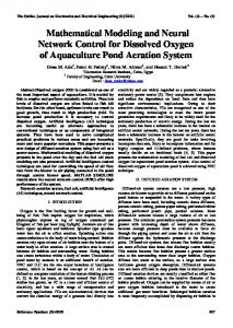
13 regression supposes a subtractive strategy, and there are two cases: neuron or input testing. As opposed to the test “2”, this new test is interesting for input testing, because it does not necessitate the training of all the submodels with fewer inputs. It is less interesting than test “2” for neuron testing, because it necessitates as many tests as there are hidden neurons, whereas test “2” necessitates only one test (see Figure 2). Moreover, it is very unlikely that a particular neuron has no significant contribution to the output after training. Actually, the same remark can be made for the pruning methods OBS and OBD, which are related to tests involving a single training, but without the notion of risk (see [Anders 1997] and Appendix 2). This Fisher test hence involves only the training of the unrestricted model with q parameters. In the following, this test will be called test “1”. IV.2.2.3. Constraints on the choice of a full model We have just seen that neural networks with one layer of hidden neurons and a linear output neuron are relatively easy to compare with hypothesis tests because they are nested models. We have briefly recalled two tests to select the simplest nested model needed to estimate the regression, given the data set. An important issue is how to choose the most complex model where to start the tests from, the “full model”. The full model must satisfy two conditions: a) according to the assumptions needed to perform statistical tests, the full model should be complex enough to provide a good approximation of the regression in the input domain delimited by the data set: there should be no “lack of fit” of the regression. b) the full model should not be too complex, especially when the data set size N is small, in order to have a good estimation of the noise variance s 2 through rqT rq N – q, where rq denotes the residuals of a model with q parameters. As a matter of fact, the associated estimator is a biased estimator of s2 for finite N. The test of fit can guarantee that a given model fulfils the first condition, but it is not always possible to perform this test. The second condition is only roughly guaranteed for a model which is approved, i.e. which is well conditioned. Thus, we propose an heuristic but economic choice of a full model among the approved models, based on another estimate of their performance, an approximate leave-one-out score. IV.3. Cross validation From a theoretical point of view, the performance of a model can be defined by the expectation of its squared error according to the distribution of x in the domain D. Generally, this expectation is estimated with the mean square error on a test set independent from the training set, the mean square performance error (MSPE). If the
14 whole data set is used for training, for example because N is small, it is still possible to estimate the expectation of the squared error with a cross-validation score. In [Rivals & Personnaz 1999], we have shown that the leave-one-out cross validation score is biased, and hence that it often does not lead to an optimal selection. Thus, we do not use leave-one-out scores for selection. But we use it as a tool to choose the full model for the tests. More precisely, we propose to use an approximate leaveone-out score. As a matter of fact, we have shown [Rivals & Personnaz 2000a] that a useful approximation of the k-th leave-one-out error is: rk ek ≈ k=1 to N (12) 1 – pz kk where pz = z z T z -1 z T denotes the (N, N ) orthogonal projection matrix on the range of the (N, q) Jacobian matrix z . Hence the approximate leave-one-out score (ALOOS):
ALOOS = 1 N
N
∑
ek 2
(13)
k=1 if z T
The ALOOS can be reliably computed only z is well-conditioned; if not, some of the diagonal terms pz kk of the projection matrix may be outside their theoretical bounds [1/N; 1]. The full model is then chosen as the approved model for which the first minimum of the ALOOS is achieved if there is one, or else as the largest approved model. The full model can be considered as a good estimate of the regression if the ratio of its N ALOOS to its mean square training error MSTE = 1 ∑ ypk – f x k , qLS 2 is close to N k =1 one. Another performance measure could be chosen (a 10-fold cross validation score, a mean square error on an independent set, etc.): the advantage of the ALOOS is that it is computed on the whole data set, and that it can be approximated in the above economic fashion.
V. PROPOSED PROCEDURE We address the problem of constructing the best neural model given a finite data set. We recall that it is assumed that x contains all the inputs necessary to “explain” E Yp . These inputs may have been roughly preselected among a list of potentially explanatory inputs, for instance by building a polynomial model. This construction can be performed step by step with an orthogonalization procedure [Chen & Billings 1989], by ranking the monomials of the elements of the list according to their relevance; the inputs involved in the first relevant monomials only are kept [Urbani et al. 1994]. This preselection may be most useful in the case of numerous potentially relevant inputs, like when predicting the solubility of pharmaceutical compounds from
15 a list of hundreds of features of the compounds molecular structure, whereas a dozen only are relevant. Once this preselection is performed, it can be assumed that x contains all the inputs necessary to “explain” E Yp , although some of them may still be superfluous. We then propose the following neural model construction and selection procedure, according to analysis performed in the previous sections. Since networks with a single hidden layer of neurons with hyperbolic tangent activation function and a linear output neuron possess the universal approximation property, we choose not to consider more complex architectures, i.e. networks with multiple hidden layers and/or a different connectivity. Hence, the determination of the best network architecture reduces to that of the best number of hidden neurons and of the relevant inputs. We propose the following procedure, which consists of two phases: a) An additive (or growing) estimation and approval phase of models with all the potentially relevant inputs, and an increasing number of hidden neurons. b) A subtractive (or pruning) selection phase among the approved models, which first removes the useless hidden neurons, and then, the useless inputs. V.I. Additive estimation and approval phase For the rough determination of the maximum size of the neural candidates, we advocate an additive procedure. As a matter of fact, additive procedures have at least two main advantages with respect to subtractive ones [Kwok & Yeung 1997]. First, it is straightforward to specify the initial neural network (a linear neuron), whereas for subtractive ones, one does not know a priori how many hidden neurons the initial neural neural network should have. Second, they are computationally more economical, since they do not waste most of the time training too large networks (for which it is difficult to ensure that a minimum is reached). On the basis of the analysis made in section IV.1 concerning the necessity of the good numerical conditioning of the candidate networks for their approval, we propose to stop the additive phase when the condition number of the Jacobian matrix z of the networks becomes too large. In practice, starting with a linear neuron, neural models with an increasing number of hidden neurons are trained, each of them several times with an efficient algorithm (for instance quasi-Newton or Levenberg-Marquardt) in order to increase the chance to obtain a global minimum of the quadratic cost function. For each number of hidden neurons, the model corresponding to the lowest minimum is kept. It is approved if the condition number of its Jacobian matrix z is below a fixed threshold (108 with an usual computer), and if its ALOOS can be reliably computed (both phenomena being linked with the conditioning of z ). The residuals of the approved models and their
16
ALOOS are stored for the subtractive phase. V.2. Subtractive hidden neuron and input selection phase In order to prepare the tests for the removal of possibly useless neurons and non significant inputs, this phase begins with the choice of the full model, on the basis of the ALOOS of the approved candidates: it is chosen as the largest approved model before the ALOOS starts to increase. If there are repetitions in the data, a test of fit can be performed in order to ensure that the full model gives a good estimate of the regression. If not, the ratio of the ALOOS of the full model to its MSTE is an indicator (though less reliable than the pure error) of a possible bias of the full model. V.2.1. Hidden neuron number selection The subtractive phase for the hidden neurons can be performed either (i) with the tests “2” using two estimates of the regression and hence two trainings (that of the unrestricted model, and that of the restricted one), or (ii) with the tests “1” involving only the estimate of the regression through the unrestricted model. Since the estimates, and hence the corresponding sums of squares of the residuals are already available, it is economic and straightforward to perform the test “2”, which necessitates only the computation of the Fisher ratio (9). The selection using test “1” is questionable due to the interchangeability of the hidden neurons, and would necessitate the computation of as many Fisher ratios (11) as there are hidden neurons. Thus, we propose to perform a sequence of tests “2” starting with the full model as unrestricted model, the restricted model being then taken as new unrestricted model, as long as the null hypothesis is not rejected. Then, none of the remaining hidden neurons can be decided irrelevant, and the input selection begins (the problem of the hidden neuron number selection was tackled in [Rivals & Personnaz 2000b], but without irrelevant inputs). V.2.2. Input selection Again, this selection can be performed with the two types of tests. But this time, the tests “2” (two trainings) are less economical because the models with one input removed have not been trained in the additive phase (their sums of squared residuals are not available). Whereas for tests “1”, it is only necessary to compute the Fisher ratios (11) corresponding to each input (which are not interchangeable). In the next section, we propose simulation experiments in order to judge experimentally what test should be chosen. Whatever the chosen tests, if several inputs are judged irrelevant, the less relevant
17 input according to the value of its Fisher ratio is removed (i.e. that with the lowest ratio), and the network is retrained. A new series of tests on the remaining inputs is performed, until the null hypothesis is rejected for all of them, i.e. until no input can be decided irrelevant. Note that a designer who is interested in a further gain in parsimony and in a slight reduction of the model variance is free to perform additional tests “1” on each parameter corresponding to an input - hidden neuron connection of the remaining fully connected network. Finally, in the absence of an independent and reliable estimate of the noise variance, the ratio of the A L O O S of the final model to its M S T E is an indicator of its performance. The closer the ratio is to one, the more likely it is that the model output is a good approximation of the regression.
VI. SIMULATION EXPERIMENTS We consider three different processes. Process #1 is a single input process simulated with:
y pk = sinc 10 (x k + 1) + w k
(14)
where “sinc” denotes the cardinal sine function. The input values x k are drawn from an uniform distribution in [–1; 1], and the noise values w k from a gaussian distribution with s 2= 2 10-3. Processes #2 and #3 are taken from [Anders & Korn 1999] in order to allow numerical comparisons of our method to those described in this recent paper on model selection. Process #2 possesses three inputs and is simulated with:
y pk = 1 + tanh 2 x 1k – x 2k + 3 x 3k + tanh x 2k – x 1k + w k
(15)
Actually, the values of the parameters of process #2 are not given in [Anders & Korn 1999]; we chose the above values so that the regression cannot be well approximated with a single hidden neuron network. Process #3 possesses two inputs and is simulated with:
y pk = – 0.5 + 0.2 x 1k 2 – 0.1 exp x 2k + w k
(16)
Their input values x ik are drawn from gaussian distributions with unit variance, and the noise values from a gaussian distribution whose standard deviation equals 20% of the unconditional standard deviation of the output, i.e. s 2 = 0.2 for process #2 and s 2 = 5 10-3 for process #3.
18 Neural networks candidates with one layer of h "tanh" hidden neurons and a linear output neuron are considered, except the network without hidden neurons which consists of a single linear neuron. For the sake of clarity, we will first present the results obtained without superfluous inputs in section VI.1. Section VI.2. then presents the input selection. VI.1. Hidden neuron number selection We build 1000 data sets of size N with different values of the noise, the input values remaining unchanged. A large separate set of 500 examples is used for the performance estimation only. The neural models are trained with the LevenbergMarquardt algorithm, each of them being trained q (the number of its parameters) times starting from different random initial parameters values, in order to increase the chance to reach an absolute minimum. Following the proposed procedure, the additive estimation and approval phase is stopped when either the condition number of z reaches 108 , or some of the diagonal terms pz kk of the projection matrix needed for the computation of the ALOOS are outside the theoretical bounds [1/N; 1]. The full model is chosen as the largest approved model before the ALOOS starts to increase, and the subtractive test phase is performed at the 5% risk level. In each case, i.e. for a given process and a fixed data set size N, we give the mean values on the 1000 data sets of: a) the number of hidden units of the full model hfull ; b) the number of hidden units of the selected model hsel ; c) the mean square training error MSTE of the selected model; d) the approximate leave-one-out score ALOOS of the selected model; e) the ratio of the ALOOS of the selected model to its MSTE , which we expect to indicate that selected model gives a good estimate of the regression when it is close to 1: p = ALOOS (17) MSTE f) the mean square performance error MSPE, i.e. the mean square error obtained on the large separate set with 500 input-output pairs; g) the relative difference in MSPE between the true model, i.e. the model whose output is the regression, and the selected model: MSPE – MSPE true model r= (18) MSPE true model Though this ratio carries the same information as the MSPE together with the noise variance s2, we use it in order to perform comparisons with the results of [Anders & Korn 1999]. Note also that, when r = 100%, the MSPE is only twice as large as s2, a value which is quite satisfactory in the case of a small data set and a complex regression.
19 The results obtained for the modeling of process #1 are shown in Table 1. In real life, the values of the MSPE and of r are not available, hence the grey background used for them in the result tables. For large N, the procedure leads to an average selected number of hidden neurons hsel of 4.2 with an average MSPE ( MSPE) equal to the noise variance, performance which indicates that this selection is adequate. Both the MSPE and hsel remain almost constant until N becomes too small with respect to the number of parameters needed for the 4 hidden units network (q = 13): hsel then drops to 3.1 for N = 50. Nevertheless, the performance is not bad (the MSPE equals twice the noise variance), and the value of the ratio p, on the average equal to 1.64, helps the designer in individual cases to diagnose that the data set size N is too small to achieve a perfect modeling. Finally, we note that, whatever N , the full model is frequently selected (hfull ≈ hsel ). The results obtained for the modeling of process #2 are shown in Table 2. By construction, the family of the neural networks with two hidden neurons contains the regression. It is interesting to note that hsel almost does not vary with the data set size N: the model with the right architecture is nearly always chosen. Like for process #1, we note that the preselection performed on the basis of the conditioning number of z and of the ALOOS almost always leads to the right model. Finally, the fact that a parameter from the input x3 to one of the hidden neurons is not necessary (see the expression (15) of the regression) does not lead to the ill-conditioning of 2 hidden units models with all their connections. The results obtained on this example can be compared to those presented in [Anders & Korn 1999], a paper which studies how hypothesis tests, information criteria and cross-validation can guide model selection; it concludes that approaches based on statistical tests lead to the best results. These approaches proceed by constructing models with an increasing number of hidden neurons, until an additional one is shown to be statistically not significant; Wald tests are then performed on the input connections. The best method described in [Anders & Korn 1999] achieves a performance which is similar to ours (rAnders = 3.3%), with roughly the same average number of hidden units of the selected model, in the case N = 500 (smaller training sets are not considered in [Anders & Korn 1999]). The results obtained for the modeling of process #3 are shown in Table 3. The regression being quite complex (see the regression surface shown in [Anders & Korn 1999]), the performance deteriorates when the size of the training set becomes too small. Again, the average numbers of hidden neurons of the full model and of the selected model increase as the data set size N increases, and the tests reduce only
20 slightly (in the average) the size of the selected model as compared to that of the full model. But this reduction is very important in the case of a small data set: as a matter of fact, the full model achieves rfull = 2.7% for N = 500 (instead of 2.5% for the selected model) and rfull = 11.6% for N = 200 (instead of 11.0%), but rfull = 1151% for N = 100 (instead of 176%). In the case N = 500, the best statistical selection method described in [Anders & Korn 1999] obtains a poor performance (rAnders = 30.9%) as compared to ours (r = 2.5% for N = 500 and also r = 11.0% for N = 200), but with roughly the same average number of hidden neurons (3.2). This difference may be due to the fact that the training algorithm of [Anders & Korn 1999] is not efficient enough, or that their Wald tests have lead to the suppression of too many connections from the inputs to the hidden neurons: on the average, 7.3 such connections remain in their selected network, whereas a completely connected 3 hidden units model possesses 9, and a 4 hidden units model possesses 11. [Anders & Korn 1999] also report that 10-fold cross-validation achieves r = 53.6% with 3.7 hidden units on the average (again with N = 500). VI.2. Hidden neuron number and input selection In order to dissociate the two problems, i.e. that of hidden neuron selection, and that of input selection, we will now consider the input selection on the models with the number of hidden neurons which is the most frequently selected, and study the performance of the two Fisher tests for the input selection when an irrelevant input exists. The irrelevant inputs values have the same distribution as the relevant ones; they have no influence on the output of the simulated process. The tests are performed at the 5% level. For process #1 with one input, we choose a training set size of N = 100. When adding 1 irrelevant input, models with 4 hidden neurons are selected at 74% by the previous procedure (IV.1), with the average performance given in Table 4. For the models with 4 hidden neurons, both tests perform well for the input selection, but the results of the tests ‘2’ are closer to those expected according to the risk level of 5% (and hence 5% of rejection of the null hypothesis). For process #2 with three inputs, we choose a training set size of N = 100. When adding 1 irrelevant input, models with 2 hidden neurons are selected at 89%, with the average performance given in Table 6. For these models, both tests perform well for the input selection, as shown in Table 7, the results are close to the expected 5% of rejection of the irrelevant input.
21 For process #3 with two inputs, the most complex one, we choose a training set size of N = 200. When adding 1 irrelevant input, models with 3 hidden neurons are selected at 84%, with the average performances given in Table 8. For these models, the test “2” still performs very well, but the test “1” performs less well. As a matter of fact, it suppresses a relevant input 7.3% of the time. However, it suppresses x1, which is less relevant than x2. Taking N = 500 does not help: it leads to 9.4% of removal of the input x1. VI.3. Discussion We can now make several statements and comments: a) The full model is often quite small, i.e. the approval based on the conditioning of z together with the rule involving the ALOOS lead to a good preliminary selection; unnecessarily complex models are not taken into account, as opposed to pruning approaches, hence sparing a lot of computation time. b) But the tests help a lot when the data set size is small. c) The ratio p = ALOOS/MSTE gives indeed a reliable indication of whether the selected model gives a good estimate of the regression, and hence if it makes sense to compute confidence intervals on its basis for example. d) The test "2" seems a little more reliable than the test “1” for input selection in the case of a complex process. This is probably due to the fact that the test "1" uses an estimate of the parameter covariance matrix which is very sensitive to the curvature of the solution surface, whereas test "2" does not.
VII. APPLICATION TO REAL WORLD MODELING PROBLEMS We selected two problems among the four regression problems proposed as benchmarks at the NIPS2000 workshop "Unlabeled data supervised learning competition", for which we obtained the highest scores using the proposed procedure. These are real world problems, and at the time of the competition, their exact nature, i.e. that of their inputs, remained secret1.
1 See: http://q.cis.uoguelph.ca/~skremer/NIPS2000/ for further details concerning the highest scores
and about the data. One of the goals of the competition was to show whether the use of unlabeled data could improve supervised learning, so in addition to the training and test sets, an addititional unlabeled set was available; however, we did not use this set to obtain the presented results.
22 VII.1. Molecular solubility prediction (problem 8 of NIPS2000) This problem involves predicting the solubility of pharmaceutical compounds, based on the properties of the compound's molecular structure. Aqueous solubility is a key in understanding drug transport, and the resulting model would be used to identify compounds likely to possess desirable pharmaceutical properties. The proposed inputs build a list of 787 real-valued descriptors, which are one-dimensional, twodimensional and electron density properties of the molecules. Thus, this is a 787 inputs, single output problem. The training set contains 147 examples, and a test set contains 50 examples. The size of the list of inputs is so high with respect to the size of the training set, that a preliminary the selection of the potentially relevant ones is mandatory. VII.1.1. Polynomial modeling The number of inputs being very large, polynomials of increasing degree but without cross-product terms are built (the latter would require too large a memory). For each degree, the polynomial with the lowest LOOS is selected2. The final polynomial is selected on the basis of the ratio p of the LOOS to the MSTE of these polynomials of different degree. This leads to the selection of the polynomial of degree 3 with 6 monomials: x 17 2, x 36, x 159, x 172 2, x 222 3, and x 565 3. Table 10 summarizes the results obtained with this polynomial3. The ratio of the LOOS to the MSTE of the selected polynomial is close to 1. Note that the size of the test set being small (50 examples), the performance is not necessarily well estimated with the MSPE. VII.1.2. Neural modeling There are 6 primary inputs involved in the monomials selected above: x 17, x 36, x 159, x 172, x 222 and x 565. They are fed to neural networks with one layer of an increasing number of hidden neurons with a "tanh" activation function, and a linear output neuron. The results of this neural modeling are shown in Table 11. The networks with more than 2 hidden neurons are not approved: the condition number of their Jacobian matrix z is larger than 108. According to a test “2” of the usefulness of the hidden neurons with risk 5%, the network with 2 hidden neurons is selected. Tests “1” as well as tests “2” lead to consider that all 6 inputs are significant. The performance of the selected network is
2 For models that are linear in the parameters, expressions (12) and (13) are exact. 3 The value of the MSPE corresponds to the squared inverse of a score of 1.382578 we obtained after
the competition, thanks to the use of the LOOS; during the competition, we obtained a score of 1.376846, which was the highest score at that time.
23 presented in Table 12. It is a little better than that of the best polynomial since its
MSPE equals 4.17 10 -1 instead of 5.23 10-1. However, the test set consisting of only 50 examples, this improvement is not necessarily significant. VII.1.3. Discussion This example is a typical illustration of the necessity of using a polynomial input selection procedure, before using neural networks. It also illustrates the fact that, when the training set is small, a neural network shows only little advantage over a polynomial. However, if more data could be gathered (in this case, the solubility of additional compounds), it is likely that neural networks would become really advantageous with respect to polynomials. VII.2. Prediction of the value of a mutual fund (problem 3 of NIPS2000) This problem consists of predicting the value of a mutual fund given the values of five other funds of a popular Canadian bank. The values were taken at daily intervals for a period of approximately three years, weekends and holidays excluded. If a good model could be built from this data, it would confirm that one mutual funds price is related to the other. This is a quite reasonable assumption because the commodities in which they invest are the same, and because general economic trends (boom/bust) affect all funds. Thus, this is a 5 inputs, single output problem. The training set contains 200 examples, as well as the test set. The number of inputs being small, neural networks can be used right away (no preliminary polynomial input selection). Table 13 summarizes the results obtained when training networks with an increasing number of hidden neurons on the whole data set, using the proposed neural network selection procedure. The networks with more than 4 hidden neurons are not approved, because of the large condition number of their Jacobian matrix z. According to a test "2" with risk 5%, the 4 hidden neuron network is selected. Further tests "1" or tests "2" performed on the inputs show that all the 5 initial inputs are significant. Table 14 presents the results4 obtained with the selected network.
VIII. CONCLUSION We have proposed an original model construction and selection procedure for neural
4 The value of the MSPE corresponds to the squared inverse of the score of 8.982381 we obtained at
the competition, which is the highest score.
24 networks. It is based on three tools: the Jacobian matrix conditioning analysis, hypothesis tests and cross validation scores obtained without trainings, and whose use we have justified at the different stages of the procedure. Thanks to the illconditioning detection, the procedure is essentially an additive one, and hence avoids the problems linked to overfitting and more generally to the use of too large networks. The statistical tests together with the cross validation scores then provide a sound basis for the removal of irrelevant neurons and inputs. The large scale simulation experiments and the real world modeling problems presented in the paper show the efficiency of the proposed procedure.
APPENDIX 1. GEOMETRICAL DEMONSTRATION FOR THE TEST OF FIT For the simplicity of the presentation, this original geometric demonstration is presented for a linear model (q = n, z = x = x1 x2 … xn , where the xi are N-vectors); under mild regularity conditions, the asymptotic results in the nonlinear case follow immediately. A training set with repetitions is available. Let M denote the number of different values of the inputs, Nk the number of repetitions at xk (k=1 to M). We denote by ypk, j the value of the process output for the jth repetition at xk (for j=1 to Nk), and ypk the M mean of the process outputs at x k . The vector of the N = ∑ Nk outputs of the =1 M,NM T training set is denoted by yp = yp1,1…yp1,N1 yp2,1 … yp1,N2 … ypM,1 k… yp , and the Nvector composed of the repeated outputs y k = x k T qLS of the linear LS model for corresponding inputs is denoted by y. In the Euclidean space of dimension N, let us consider the M > n orthogonal vectors e i i=1 to M such that: – the N1 first components of the vector e1 are equal to one and the others to zero; – the components N1+1 to N1+N2 of the vector e 2 are equal to one and the others to zero; – … – the NM last components of the vector eM are equal to one and the others to zero. We define LM as the subspace of dimension M spanned by these vectors. Thus, the regressor vectors xi , i=1 to n belong to L M . In other words, the subspace Ln spanned by the columns of x belongs to LM (see Figure A1.1). Since the vector of the outputs of the linear model y = x qLS is a linear combination of the xi , it also belongs to LM. The orthogonal projection matrix on the subspace spanned by a vector e i is e i e iT Ni.
25 Since the vectors e i i=1 to M are orthogonal, the orthogonal projection matrix on LM is M ∑ e i e iT Ni. The orthogonal projection ypM of yp onto the subspace LM is hence: i=1
M
ypM = ∑ i=1
ypi
ei , where
ypi
=1 Ni
Ni
∑ ypi,j
(A1.1)
j=1
By definition, the residual vector is r = yp – y , the pure error vector is p = yp – ypM , and the model error vector is m = ypM – y .Taking the previous orthogonality into account, we obtain (see Figure A1.1):
r T r = p T p + m T m = ssrpe + ssrme
(A1.2)
Let us define the null hypothesis H 0 as the hypothesis that the model contains the regression, i.e. that the subspace Ln spanned by the columns of x contains E Y p . If H0 is true, the expectation of M is zero, and the residual vector r is the orthogonal projection of the noise vector w onto the subspace orthogonal to Ln . Furthermore, if the measurements are homoscedastic and gaussian with variance s 2, the normalized vector W s →N 0 , IN is the sum of three orthogonal projections, whose squared norms are independent c2 variables (Fisher-Cochrane theorem): W = P + M + E (Y p) – Y (A1.3) s s The first two squares are SSR pe s 2 and SSR me s 2, which are c 2 distributed with respectively N–M and M–n degrees of freedom. The ratio u: m T m / (M – n) ssrme / (M – n) u= = (A1.4) p T p / (N – M) ssrpe / (N – M) is hence the realization of a random variable which is Fisher distributed with M–n and N–M degrees of freedom. Hence the Fisher test of fit.
APPENDIX 2. STATISTICAL INTERPRETATION OF PRUNING METHODS In the case of the test of a single parameter, i.e. of the null hypothesis qpi = 0, the relation (11) becomes: qLSi 2 N – q u (1) = (A2.1) z T z -1 ii rqT rq u (1) is here the value of a random variable approximately Fisher distributed, with 1 and N – q degrees of freedom. Equivalently, u (1) = qLSi N – q z T z -1 ii rqT rq is the value of a random variable approximately Student distributed, with N – q degrees of freedom. It is worth mentioning the link of this test to the pruning methods such as OBD (for Optimal Brain Damage, see [Le Cun et al. 1990]) or OBS (for Optimal Brain Surgeon [Hassibi & Stork 1993]). As a matter of fact, both methods use a measure of the saliency of the parameters which is close to the ratio u (1) (see [Anders 1997]).
26 A2.1. The pruning method OBD The pruning method OBD estimates the variation ∆Ji of the cost function J qLS due to the nullification of the ith-parameter by using a quadratic approximation of the cost function at the minimum, and by neglecting the non diagonal terms of the Hessian h of the cost function: ∆Ji = 1 h ii qLSi 2 (A2.2) 2 The smaller ∆Ji, the less relevant the corresponding ith-parameter is considered by OBD. The method consists in choosing an initial neural model that is “sufficiently large” (note that it would be better to talk about a full model, as defined by us previously; it would also be preferable to choose it with the tools we have proposed, rather than randomly choosing a large network which may be totally ill-conditioned, and whose Hessian hence cannot be computed accurately), and to perform the following procedure: 1) Minimize the quadratic cost function; 2) Compute the ∆Ji and suppress the connections whose ∆Ji are below a given threshold; 3) Go back to 1 or stop the procedure if a stopping criteria is satisfied. The reader will have noted the similarity between (A2.1) and the ratio u (1) (A2.2) used in the test "1". As a matter of fact, if the Hessian is approximated by its diagonal, we have h ii ≈ 1 h -1 ii, and the Hessian asymptotically tends to the squared Jacobian z T z . But there are two differences: – test "1" does not approximate the squared Jacobian through its diagonal; – as opposed to test "1", whose ratio u (1) includes a normalization through rqT rq N – q, and which supplies a threshold for the value u (1) that is a function of the risk taken, OBD does not give a threshold on ∆Ji for the removal of the parameters. A2.2. The pruning method OBS The OBS method, an improved version of OBD, is based on the suppression of the parameter for which the following quantity is the smallest: q 2 (A2.3) ai = 1 LSi 2 h -1 ii and proposes a modification of the other parameters that leads to the smallest possible increase of the cost function. This modification being computed with a quadratic approximation of the cost function, it is actually necessary to retrain the network in order to find the optimal value of the remaining parameters. The main advantage of OBS is not to consider the Hessian as diagonal, which makes the ai even closer to the ratio u (1). But, like OBD, OBS does not specify a threshold
27 for the removal of the parameters. To conclude, the pruning methods OBS and OBD are indeed related to test "1", but the notion of risk is absent, and thresholds must be set in an ad hoc fashion: they are hence less likely to succeed in the pruning of irrelevant neurons or inputs than test "1".
ACKNOWLEDGEMENTS
We are very grateful to Stefan S. Kremer and to the organisers of the NIPS2000 workshop “Unlabeled data supervised learning competition”.
REFERENCES U. Anders, “Neural network pruning and statistical hypotheses tests,” in Progress in Connectionnist-Based Information Systems (Addendum), Proceedings of ICONIP’97. Berlin: Springer, 1997, pp. 1-4. U. Anders and O. Korn, “Model selection in neural networks,” Neural Networks, vol. 12, pp. 309-323, 1999. A. Antoniadis, J. Berruyer, and R. Carmona, Régression non linéaire et applications. Paris: Economica, 1992. D. M. Bates and D. G. Watts, Nonlinear regression analysis and its applications. New York: Wiley, 1988. M. Bishop, Neural Networks for Pattern Recognition. Oxford: Clarendon Press, 1995. W. Buntine and A. Weigend, “Computing second derivatives in feedforward neural networks: a review,” IEEE Transactions on Neural Networks, vol. 5, pp. 480-488, 1994. S. Chen, A. Billings, and W. Luo, “Orthogonal least-squares methods and their application to non-linear system identification,” Int. J. of Control, vol. 50, pp. 1873-1896, 1989. B. Efron and R. J. Tibshirani, An introduction to the bootstrap. New York: Chapman & Hall, 1993. S.E. Fahlman and C. Lebière, “The cascade correlation learning architecture,” in Advances in Neural Information Processing Systems 2. San Mateo, CA: Morgan Kaufman, 1990, pp. 524-532. J. H. Friedman, “An overview of predictive learning and function approximation,” in
28
From Statistics to Neural Networks: Theory and Pattern Recognition Applications, J. H. Freidman and H. Wechsler, Eds. ASI Proc., Subseries F. New York: Springer-Verlag, 1994. G. H. Golub and C. F. Van Loan, Matrix computations. Baltimore: The John Hopkins University Press, 1983. G. C. Goodwin and R. L. Payne, Dynamic system identification; experiment design and data analysis. New York: Academic Press, 1977. L. K. Hansen and J. Larsen, “Linear unlearning for cross validation,” Advances in computational mathematics vol.5, pp. 296-280, 1993. B. Hassibi B. and D. G Stork, “Second order derivatives for network pruning: optimal brain surgeon,” in Advances in Neural Information Processing Systems 5. San Mateo, CA: Morgan Kaufmann, 1993, pp. 164-171. B. Hassibi, D. Stork, G. Wolff, and T. Watanabe, “Optimal brain surgeon: Extensions and performance comparisons,” in Advances in Neural Information processing Systems 6. San Mateo, CA: Morgan Kaufman, 1994, pp. 263-270. T. Heskes, “Practical confidence and prediction intervals,” in M. Mozer, M. Jordan & T. Petsche (Eds.), Advances in Neural Information Processing Systems 9 . Cambridge, MA: MIT Press, 1997, pp. 176-182. T. Y. Kwok and D. Y. Yeung, “Constructive algorithms for structure learning in feedforward neural networks for regression probems,” IEEE Trans. Neural networks vol. 8, pp. 630-645, 1997. Y. Le Cun, J. S. Denker, and S. A. Solla, “Optimal brain damage,” in D. S. Touretzki (Ed.), Advances in Neural Information Processing Systems, vol. 2. San Mateo, CA: Morgan Kaufmann, 1990, pp. 598-605. I. J. Leontaritis and S. A. Billings, “"Model selection and validation methods for nonlinear systems,” Int. J. Control, vol. 45, pp. 311-341, 1987 D. J. C. MacKay, “Bayesian interpolation,” Neural computation, vol. 4, pp. 415-447, 1992. D. J. C. MacKay, “A practical Bayesian framework for backprop networks,” Neural computation, vol. 4, pp. 448-472, 1992. D. J. C. MacKay, “Comparison of approximate methods for handling hyperparameters,” Neural computation, vol. 11, pp. 1035-1068, 1999. M. Minoux, Programmation mathématique; théorie et algorithmes. Paris: Dunod, 1983. J. Moody, “Prediction risk and architecture selection for neural networks,” in From statistics to neural networks: theory and pattern recognition applications. NATO ASI Series, Springer Verlag, 1994. G. Paass, “Assessing and improving neural network predictions by the bootstrap
29 algorithm,” In S. J. Hanson, J. D. Cowan, & C. L. Giles (Eds.), Advances in Neural Information Processing Systems , vol. 5. Cambridge, MA: MIT Press,1993, pp. 186-203. W. H. Press, S.A. Teukolsky, W. T. Vetterling, and B. P. Flannery, Numerical recipes in C. Cambridge: Cambridge University Press, 1992. R. Reed, “Pruning algorithms–A review,” IEEE Trans. Neural Networks, vol. 4, pp. 740-747, 1993. A.-P. N. Refenes, A. D. Zapranis, and J. Utans J., “Neural model identification, variable selection and model adequacy,” In Decision technologies for financial engineering, A. S. Weigend, Y. Abu-Mostafa, A.-P. N. Refenes eds. World scientific, 1997, pp. 243-261. B. D. Ripley, Pattern recognition and neural networks. Cambridge: Cambridge University Press, 1995. I. Rivals and L. Personnaz, “Construction of confidence intervals in neural modeling using a linear Taylor expansion,” in Proceedings of the International Workshop on Advanced Black-Box Techniques for Nonlinear Modeling, 8-10 July 1998, Leuwen, pp. 17-22. I. Rivals and L. Personnaz, “On cross-validation for model selection,” Neural Computation, vol. 11, pp. 863-870, 1999. I. Rivals I. and L. Personnaz, “Construction of confidence intervals for neural networks based on least squares estimation,” Neural Networks, vol. 13, pp. 8090, 2000. I. Rivals I. and L. Personnaz, “A statistical procedure for determining the optimal number of hidden neurons of a neural model,” in Proceedings of the Second International Symposium on Neural Computation (NC’2000), May 23-26 2000. S. Saarinen, R. Bramley; and G. Cybenko, “Ill-conditioning in neural network training problems,” SIAM J. Sci. Stat. Comp., vol. 14, pp. 693-714, 1993. G. A. F. Seber, Linear regression analysis. New York: Wiley, 1977. G. A. F. Seber and C. Wild, Nonlinear regression. New York: Wiley, 1989. H. J. Sussman, “Uniqueness of the weights for minimal feedforward nets with a given input-output map,” Neural Networks, vol. 5, pp. 589-593, 1992. D. Urbani, P. Roussel-Ragot, L. Personnaz, and G. Dreyfus G., “The selection of neural models of non-linear dynamical systems by statistical tests,” in Neural Networks for Signal Processing, Proceedings of the 1994 IEEE Workshop, 1994. H. White, “Learning in artificial neural networks: a statistical perspective,” Neural Computation, vol. 1, pp. 425-464, 1989. G. Zhou and J. Si, “A systematic and effective supervised learning mechanism based on Jacobian rank deficiency,” Neural Computation, vol. 10, pp. 1031-1045, 1998.
30
TABLES Table 1. Neuron selection results for process #1 (s 2 = 2 10-3).
N
hfull
hsel
50 100 200 500
3.2 4.2 4.3 4.3
3.1 4.1 4.2 4.2
MSTE 1.94 10-3 1.77 10-3 1.86 10-3 1.94 10-3
ALOOS 3.08 10-3 2.39 10-3 2.15 10-3 2.05 10-3
p 1.64 1.35 1.15 1.06
MSPE 4.40 10-3 2.56 10-3 2.28 10-3 2.1410-3
r 108.4% 15.9% 8.2% 3.1%
Table 2. Neuron selection results for process #2 (s 2 = 2 10-1).
N
hfull
hsel
50 100 200 500
2.1 2.2 2.2 2.2
2.0 2.1 2.1 2.2
MSTE 1.59 10-1 1.73 10-1 1.86 10-1 1.94 10-1
ALOOS 2.69 10-1 2.23 10-1 2.10 10-1 2.03 10-1
p 1.75 1.30 1.10 1.05
MSPE 2.89 10-1 2.23 10-1 2.01 10-1 1.92 10-1
r 44.2 % 18.3% 8.4% 3.1%
Table 3. Neuron selection results for process #3 (s 2 = 5 10-3).
N
hfull
hsel
100 200 500
3.2 3.3 3.4
3.1 3.2 3.3
MSTE 4.48 10-3 4.64 10-3 4.82 10-3
ALOOS 7.20 10-3 5.74 10-3 4.15 10-3
p 1.6 1.2 1.1
MSPE 1.38 10-2 5.79 10-3 4.41 10-3
r 176% 11.0% 2.5%
Table 4. Neuron selection results for process #1 with 1 irrelevant input (N = 100, s 2 = 2 10-3): 74% of the selected models have 4 hidden neurons.
N
hfull
hsel
100
4.1
4.0
MSTE ALOOS 1.80 10-3 2.63 10-3
p 1.48
MSPE 2.77 10-3
r 32.3%
Table 5. Input selection results for process #1 with 1 irrelevant input and 4 hidden neurons (N = 100, s2 = 2 10-3). Removed input
None
Relevant input
Irrelevant input
Test “1” Test “2”
2.1% 5.5%
0.0% 0.0%
97.9% 94.5%
31 Table 6. Neuron selection results for process #2 with 1 irrelevant input (N = 100, s 2 = 2 10-1): 89% of the selected models have 2 hidden neurons.
N
hfull
hsel
100
2.1
2.1
MSTE ALOOS 1.70 10-1 2.29 10-3
p
r
MSPE 2.34 10-1
1.36
23.8%
Table 7. Input selection results for process #2 with 1 irrelevant input and 2 hidden neurons (N = 100, s2 = 2 10-1). Removed inputs
None
Relevant input
Irrelevant input
Test “1” Test “2”
5.1% 6.4%
0.0% 0.0%
94.9% 93.6%
Table 8. Neuron selection results for process #3 with 1 irrelevant input (N = 200, s 2 = 5 10-3): 84% of the selected models have 3 hidden neurons.
N
hfull
hsel
100
3.2
3.2
MSTE ALOOS 4.54 10-3 5.85 10-3
p
r
MSPE 6.02 10-3
1.29
15.3%
Table 9. Input selection results for process #3 with 1 irrelevant input and 3 hidden neurons (N = 200, s2 = 5 10-3). Removed inputs
None
Relevant input
Irrelevant input
Tests “1” Tests “2”
1.1% 6.7%
7.3% 0.0%
91.6% 93.3%
Table 10. Preliminary selection of the potentially relevant inputs among the list of 787 for the molecular solubility prediction (problem 8 of NIPS2000): performance and features of the selected polynomial. Degree
Number of monomials
MSTE
LOOS
p
MSPE
3
6
2.66 10-1
2.89 10-1
1.1
5.23 10-1
Table 11. Neural modeling for the molecular solubility prediction (problem 8 of NIPS2000): additive phase for neural models with 6 inputs.
h
MSTE
ALOOS
k z
0 1 2 3
3.77 10-1 3.60 10-1 2.41 10-1 2.03 10-1
4.77 10-1 4.50 10-1 3.48 10-1 –
5.8 6.4 1.2 102 1.5 1018
32 Table 12. Neural modeling for the molecular solubility prediction (problem 8 of NIPS2000): performance and features of the selected network.
n
h
MSTE
ALOOS
6
2
2.41 10-1
3.48 10-1
p 1.44
MSPE 4.17 10-1
Table 13. Neural modeling for the prediction of the value of a mutual fund (problem 3 of NIPS2000): additive phase for neural models with 5 inputs.
h
MSTE
ALOOS
k z
0 1 2 3 4 5
7.22 10-2 4.60 10-2 2.13 10-2 1.38 10-2 1.07 10-2 8.14 10-3
7.74 10-2 5.16 10-2 3.06 10-2 1.82 10-2 1.75 10-2 1.47 10-2
5.9 1.2 102 2.9 102 6.8 102 5.3 102 3.0 108
Table 14. Neural modeling for the prediction of the value of a mutual fund (problem 3 of NIPS2000): performance and features of the selected network.
n
q
MSTE
ALOOS
4
29
1.07 10-2
1.75 10-2
p 1.63
MSPE 1.24 10-2
33
FIGURES
∑
ƒ ∑
ƒ ∑
x1
ƒ ∑
x2
Unrestricted model (q parameters) ∑
∑ ƒ ∑
ƒ ∑
x1
x2
Restricted model for testing whether two hidden neurons are sufficient
ƒ ∑
ƒ ∑
∑
ƒ ∑
x2 Restricted model for testing whether input x1 is significant
ƒ ∑
ƒ ∑
ƒ ∑
x1 Restricted model for testing whether input x2 is significant
Restricted models (q' parameters) Figure 1. Unrestricted and restricted models for tests involving two trainings (tests “2”).
34
Restricted models (their parameters do not need to be estimated)
Unrestricted model (q parameters) ∑
ƒ ∑
∑
ƒ ∑
x1
ƒ ∑
ƒ ∑
x2
∑
ƒ ∑
x1
ƒ ∑
x2
ƒ ∑
x2
x2
∑
ƒ ∑
ƒ ∑
x1
ƒ ∑
Restricted model for testing whether input x2 is significant
∑
ƒ ∑
x1
ƒ ∑
x1
Restricted model for testing whether input x1 is significant
∑
ƒ ∑
x2
ƒ ∑
ƒ ∑
x1
x2
Restricted models for testing whether two hidden neurons are sufficient
Figure 2. Unrestricted and restricted models for tests involving a single training (tests “1”).
35
Choice of the full model among the approved candidates Test for lack of fit Test of the restricted model against the unrestricted one (test “2”) Remove a hidden neuron Choice of a linear model with all the possibly relevant inputs
All hidden neurons are statistically significant
No
Yes * Parameter estimation * Condition number computation * ALOOS computation Add a hidden neuron
Yes
Test of the restricted models against the unrestricted one (test “1” or test “2”) Remove the less significant input
The model is approved
No
All inputs are statistically significant
No
Yes
End
End
1) Additive phase
2) Subtractive phase
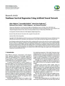
Figure 3. Proposed procedure for neural model construction and selection.
36
yp
RN
p
r
w
ypM LM
m y
E Yp
Ln
Figure A1.1. Geometrical representation of the test for fit when H0 is true, i.e. when the regression E(Yp) belongs to the subspace Ln spanned by the columns of x (Ln itself belonging to the subspace LM ).