AIML Journal, Volume (6), Issue (1), January, 2006
Neural Network Corner Detection of Vertex Chain Code S. H. Subri, H. Haron, R. Sallehuddin Department of Modeling and Industrial Computing, Faculty of Computer Science & Information Systems, University Technology of Malaysia, 81310 UTM Skudai, Johor, Malaysia
[email protected],
[email protected],
[email protected] Abstract This paper presents a Neural Network Classifier to be implemented in corner detection of chain code series. The classifier directly uses chain code which is derived using Freeman chain code as training, testing and validation set. The steps of developing Neural Network Classifier are included in this paper. Comparison results between Neural Network Classifier corner detection and other computational corner detection are presented to show the reliability of the proposed classifier. This paper ends with the discussions on the implementation of proposed neural network in corner detection of chain code series. Experimental results have shown that the proposed network has good robustness and detection performance. This makes this method a great choice for machine vision. Keywords: neural network, chain code, corner detection, line drawing
1 Introduction Corner detection is an important aspect in image processing and researchers find many practical applications in it. Corner that exists in any irregular line must be detected so that the irregular line can be interpreted to represent actual line. Corners serve to simplify the analysis of images by drastically reducing the amount of data to be processed [1]. Contours are commonly codified with the Freeman chain-code [2] where, assuming 8connectivity, eight different values are given to the eight possible neighbours of a point. The Freeman chain code consists of eight different numbers, d i ∈ {0,1,2,3,4,5,6,7}, i = 1,2,3...., n where
d i represents the position of point according to the eight possible neighbours. In this paper, contours or
regular line drawings and irregular line drawings were presented by Freeman chain-code. Many researchers’ studies show that corner detection of chain-code use computational method as their main methodology. This computational method was used by Haron [3], Ji [4] and Lee [5]. Nevertheless, very few research is done on the corner detection of chain code series based on artificial intelligence approach such as neural network and fuzzy logic. Therefore, this paper discussed a biological system which used Artificial Neural Network technique as a methodology. The neural network applied Freeman chain code directly to the network and no computational method was used in this corner detector. Artificial intelligence becomes more popular nowadays. This paper presents an Artificial Neural Network based approach to corner detection in two dimensional (2D) line drawing. The idea for initializing this neural network techniques in corner detection is based on past works which were done by Dias [6], Tsai [7] and Sanchiz [8]. However based on the research done, there was no latest further work done to enhance and improve this method. This paper is expected to lead other researchers to do research in this area. The organization of this paper is as follows. It is divided into five sections. Section (1) gives introduction, several past works and application on neural network to corner detection using chain code series. Section (2) gives details of the proposed methodology are discussed. Section (3) presents experimental result and comparison of the result with computational method. Section (4) gives conclusion and finally Section (5) presents future works.
2 Neural Network Classifier The Neural Network (NN) Classifier in this paper identifies the corner detection of 2D line drawing. The line drawing was codified to chain code using Freeman chain code and was directly used as an input of the NN
37
AIML Journal, Volume (6), Issue (1), January, 2006
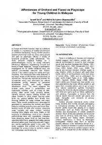
Classifier. The outputs of the NN Classifier are represented either by number 1 or 0. Number 1 represents corner. On the other hand 0 means no corner. Analysis is done to determine the best network architecture of NN Classifier. The analysis was based on trial and error. From the analysis done, the best network architecture for NN Classifier is a threelayer network model which consists of one input layer, one hidden layer and one output layer. Figure 1 shows the three-layer neural network architecture.
1 2 3
1 2
1
9
9 Figure 1: Architecture of the Neural Network Classifier This analysis is done by training the network using variation of parameter, training function and differences of network structure. Three training functions were used in this analysis. The training functions are: • Traingdx (batch gradient descent with momentum and adaptive learning rate). The function of Traingdx combines adaptive learning rate with momentum training. The performance of the algorithm is very sensitive to the proper setting of the learning rate. • Traingd (batch gradient descent backpropagation) is the batch steepest descent training function. The weights and biases are updated in the direction of the negative gradient of the performance function. • Traingdm (batch gradient descent with momentum). Momentum allows a network to respond not only to the local gradient, but also to recent trends in the error surface. Acting like a low-pass filter, momentum allows the network to ignore small features in the error surface. Traingdx and Traingdm training functions use momentum (β) for their training. The momentum is set to 0.1, 0.25, 0.5 or 0.9 while Traingd training function does not use momentum in its training. All these training function use learning rate (α) in their training. The value of this rate is set to 0.1, 0.25, 0.3,
0.5 or 0.75. The analysis was also done using variation of network structure. As shown in Table 1, 2 and 3 there are training model either with one hidden node or two hidden nodes. All hidden nodes in this analysis used LogSigmoid (Logsig) transfer function. More than 71 models were trained during the analysis. Each training functions have their best model but for the NN Classifier the best model among the three models were chosen. Table 1 shows the training model of Traingdx training function. Table 2 show the training model of Traingd training function and Table 3 shows the training model of Traingdm training function. The best model for every training function is the model whose row was shaded in each table. Among these three models, one of the models has been identified as the best model with the highest percentage of accuracy and closest condition with exact output validation. The best model is model number 20 which is in Table 1. This model uses Traingdx training function. As a threelayer network, this model only has one hidden node with nine nodes. These nine nodes were determined by using Tang and Fishwick Formula which is ‘n’ where n represents input nodes. Hidden node used Log-Sigmoid transfer function while output node used Linear transfer function. This model used feed-forward backpropagation as its network type. Mean square error (MSE) function was chosen to evaluate network performance. One value was set as a goal. All training network should be trained until the performance of the networks lower than a value of the goal. For this model, 0.01 has been chosen as a goal parameter. The other parameters of this model are learning rate (α) which was set for 0.25, momentum (β) which has been set for 0.5 and finally maximum epoch which was set for 200,000. For training models which had reached 200,000 epochs but the performance was still above the goal value, this means the network was failed. The step on how to train network and how NN Classifier is developed will be discussed in Section 2.1. 2.1 Training the Network The NN Classifier uses supervised training technique. The process of training the network consists of feeding it with a set of training samples which is provided with input and output. The input sets are pieces of chain code which are 9 codes in length for every one output which is extracted from 2D line drawing. The teaching output is a value related to the result of the input set. A total of 197 sets of input and output were involved in the training sessions while 103 sets of input and output for testing and 103 sets of input and output for validation session. A sample of 2D line drawing from Haron [9] which used computational method has been codified to chain code as an input and output set to train the network in the training session. Below are the steps taken to train the classifier.
38
AIML Journal, Volume (6), Issue (1), January, 2006
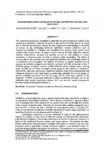
Step 1: The input and output were arranged as an array. Figure 2 shows sets of half input and Figure 3 shows set of half output. Figures 2 and 3 also show the input and output arranged in column. Step 2: Using Matlab, a network was trained using the value and parameter which have been discussed in section two. Step 3: Trained network models are tested with a sample of 103 sets of input and output. In the testing stage, accuracy and MSE output are determined. The percentage of the accuracy is based on how many trained outputs are the same with the real output. All the trained output which are the same with real output will be divided by 103 to get the accuracy percentage. The model with the highest accuracy percentage is the best network model. This model is a neural network corner detector and is known as NN Classifier.
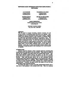
by looking at the sketch, there are 10 corners that exist along the boundary line as shown in Figure 5. Comparison results between proposed Artificial Neural Network method and computational method is shown in Table 7. Out of all 10 corners, the computational method detects 9 corners and the proposed NN Classifier detects all the corners. The corner at location 5 has not been detected by computational method. Comparison results between NN Classifier and computational method shows that NN Classifier performance is better than the computational method in terms of the number of corners detected. Columns 1 through 13 1 1 0 1 2 1 0 1 2 1 0 1 2 1 1 1 2 1 1 1 2 1 1 1 1 1 1 1 1 1 1 1 1 1 1 1 1 1 1 1 1 1 1 1 0
Step 4: The best network model is used as NN Classifier to detect corner and this corner is tested by using an image. The image has to be first codified to chain code. The chain code was arranged as an array and then it is tested with the classifier to detect corner. Experimental results are discussed in Section 3.
1 1 1 1 1 1 1 0 1
1 1 1 1 1 1 0 1 0
1 1 1 1 1 0 1 0 1
1 1 1 1 0 1 0 1 1
1 1 1 0 1 0 1 1 1
1 1 0 1 0 1 1 1 1
1 0 1 0 1 1 1 1 1
0 1 0 1 1 1 1 1 1
Columns 14 through 26 1 0 1 1 1 1 0 1 1 1 1 1 1 1 1 1 1 1 1 1 1 1 1 1 1 1 1 1 1 2 1 1 1 1 2 2 1 1 1 2 2 1 1 1 2 2 1 1 1 2 2 1 1 2
1 1 1 2 2 1 1 2 2
1 1 2 2 1 1 2 2 2
1 2 2 1 1 2 2 2 2
2 2 1 1 2 2 2 2 2
2 1 1 2 2 2 2 2 2
1 1 2 2 2 2 2 2 2
1 2 2 2 2 2 2 2 2
6 6 6 6 7 0 7 0 7
2 3 3 3 4 3 3 4 4
5 4 4 4 5 5 5 5 5
7 7 0 0 0 0 7 0 7
0 0 0 0 7 0 7 6 6
3 3 4 3 5 4 4 4 5
to Columns 183 through 195 0 1 2 2 5 6 1 0 2 2 4 6 0 1 2 2 4 7 1 0 2 3 4 7 0 1 2 3 5 0 1 1 3 3 5 0 1 0 3 4 5 0 0 0 3 3 5 0 0 1 4 3 5 7
3 Experimental Results
0 7 0 7 6 6 6 6 6
Columns 196 through 197 0 6 0 6 7 7 0 0 7 7 6 0 6 7 6 0 6 7
The classifier is tested on line drawing in Figure 4 where the chain code of the line drawing is shown in Table 4. The line drawing is taken from Haron [3]. Line drawing in Figure 4 has been codified to chaincode and the chain-code was arranged as an array in length of nine codes every one column. The chain code of the line drawing in Table 4 is a chain code of boundary list only.
Figure 2: Sets of Input Columns 1 through 13 0
As shown in Table 6, there are columns which are not the same as real output in Table 5. Column 13 and column 79 show that corner exists in each column. In the real output there was no corner in that column. However in column 102, result shows that corner does not exist but there should be a corner in that column. The result shows that NN Classifier detected 9 correct corners out of 10.
0
0
0
0
0
0
0
0
0
0
0
0
0
0
0
0
0
0
0
1
0
1
0
1
0
Columns 14 through 26 0
0
0
0
0
1
to Columns 183 through 195 0
0
0
0
1
1
1
Columns 196 through 197 0
0
Figure 3: Sets of Output
3.1 Comparison of Results In order to test the performance of the NN Classifier, the experimental results are compared to the computational method done by Haron [3]. Since the boundary line chain code is used to test the classifier, Figure 4: A Stair 39
AIML Journal, Volume (6), Issue (1), January, 2006
Table 4 Boundary List Chain Code BOUNDARY AND INTERNAL LIST List of Direction 0: Row Col Code 1 26 -1 2 27 1 3 28 1 3 29 0 4 30 1 4 31 0 5 32 1 5 33 0 6 34 1 7 35 1 7 36 0 7 37 0 8 38 1 9 39 1 10 40 1 11 41 1 12 41 2 13 41 2 14 41 2 15 41 2 16 41 2 17 41 2 18 41 2 19 41 2 20 41 2 21 41 2
22 23 24 25 26 27 28 29 30 31 32 33 34 35 35 36 37 37 37 38 38 38 39 39 39 40 40 41 42 42 43 44 44 45 44
41 41 41 41 41 41 41 41 41 41 41 40 39 38 37 36 35 34 33 32 31 30 29 28 27 26 25 24 23 22 21 20 19 18 17
2 2 2 2 2 2 2 2 2 2 2 3 3 3 4 3 3 4 4 3 4 4 3 4 4 3 4 3 3 4 3 3 4 3 5
44 44 44 43 42 41 40 39 38 37 36 35 34 33 32 31 30 29 28 27 27 27 27 27 26 26 25 24 23 22 21 20 19 18 17
16 4 15 4 14 4 13 5 12 5 11 5 10 5 9 5 8 5 7 5 6 5 5 5 4 5 4 6 4 6 4 6 4 6 4 6 5 7 6 7 7 0 8 0 9 0 10 0 11 7 12 0 13 7 13 6 13 6 13 6 13 6 13 6 13 6 13 6 14 7
17 15 0 16 16 7 16 17 0 15 18 7 15 19 0 14 20 7 13 20 6 12 20 6 11 20 6 10 20 6 9 20 6 8 20 6 7 21 7 6 21 6 5 22 7 4 23 7 3 24 7 2 25 7
tedious because it involves training samples that have to pass through three stages while the trial and error process will sometime lead to no result. This proposed method is limited for 2D line drawings only. However, this method can be applied in line drawing interpretations. It is not possible to implement this method to sketch interpreter like SILK which was developed by Landay [10] and made the sketch interpreter faster and more efficiently. The experiment shows that the optimal parameter of the classifier are alpha is equal to 0.25, and beta is equal to 0.5, and finally maximum epoch is equal to 200,000. The parameters is considered the optimal parameter after the training is conducted.
Table 5 Real Outputs Columns 1 through 13 0
0
0
0
0
0
0
0
0
0
1
1
0
0
0
0
0
0
0
0
0
1
0
0
0
0
0
0
0
0
0
0
0
0
0
0
0
0
1
0
0
0
0
0
0
0
0
0
0
1
0
0
0
0
0
0
0
0
1
0
0
0
0
0
0
1
0
Columns 14 through 26 0
0
0
0
0
Columns 27 through 39
After the chain code was arranged as an array, the boundary list in Figure 4 becomes 103 inputs. There are 10 corners found in the 103 inputs. Table 5 shows the real output and Table 6 shows output using NN Classifier to detect corner where 0 means it’s not a corner and 1 means there is a corner in that column.
0
0
0
0
0
Columns 40 through 52 0
0
0
0
0
Columns 53 through 65 0
4 Conclusions
0
0
0
0
Columns 66 through 78 0
The results show that there are advantages and disadvantages of using neural network in corner detection of chain code series. This section gives the strength and drawbacks of the method which is based on the experiments of training conducted on the network model.
0
1
0
0
Columns 79 through 91 0
0
0
1
0
Columns 92 through 103 0
The results shows that the strength of applying neural network in corner detection is it makes corner detector more sensitive in detecting a corner. That is the reason why more corners are detected using this method. Corner detection in neural network is based on pattern training sample which trained the network. Corner is detected when there is a similarity between corner chain-code trained pattern and chain code of the line drawing. The proposed method used chain code series directly without any calculation to fit it with the network. It makes this method easy to be used and applied. The chain code series just need to be arranged as an array to make it an input. The drawbacks of the this method is it can be classified as tedious and trial and error process. It is
0
0
0
1
0
Figure 5: Corner of boundary line
40
AIML Journal, Volume (6), Issue (1), January, 2006
research of fuzzy in corner detection done by Pahor [13] can be applied to detect corner of chain code series.
Table 6 Neural Network Classifier Outputs
References
Columns 1 through 13 0
0
0
0
0
0
0
0
0
0
1
1
1
[1]
0
0
0
0
0
0
0
0
[2]
1
0
0
0
0
0
0
0
[3]
0
0
0
0
0
0
0
0
0
1
0
0
0
0
0
0
[4]
0
0
0
0
1
0
0
0
[5]
0
0
0
0
0
1
0
0
0
0
0
0
0
0
Columns 14 through 26 0
0
0
0
0
Columns 27 through 39 0
0
0
0
0
Columns 40 through 52 0
0
0
0
0
Columns 53 through 65 0
0
0
0
0
Columns 66 through 78 0
0
1
0
0
Columns 79 through 91 1
0
0
1
0
Columns 92 through 103 0
0
0
0
1
0
[6]
[7]
Table 7 Comparison Table Method
No. of Corner
The Proposed NN Classifier
10
Computational Method (Haron [3])
9
5.
Corner Location 1, 2, 3, 4,5, 6, 7, 8, 9 and 10 1, 2, 3, 4, 6, 7, 8, 9 and 10
Future Works
This proposed method is a 2D line drawing corner detector. The corner detection by neural network Classifier is based on chain code series by Freeman [2]. An improvement can be done to this proposed method. The lists of the improvement are given below: •
•
[8]
[9] [10] [11] [12] [13]
Chain code techniques are widely used because they preserve information and allow considerable data reduction. In this proposed method, we use the existing Freeman chain code. Besides Freeman, chain code representation has also been proposed by Bribiesca [11, 12] to represent 2D and 3D curve. For detecting corner of these curves using NN classifer, the Vertex Chain Code (VCC) and the 3D chain code proposed by Bribiesca [11, 12] can be used to replace the Freeman chain code. Besides neural network, fuzzy logic is another one of the artificial intelligence techniques. A
.
41
H.C. Liu and M.D Srinath, Corner Detection From Chain-Code. Patt. Recognition Lett., vol. 23, pp. 51-68, 1990. H. Freeman, On the Encoding of Arbitrary Geometric Configurations, IRE Trans. On Electronic Computers, EC-10, pp. 260-268, 1961. H. Haron, S. M Shamsuddin and D. Mohamed, A New Corner Detection Algorithm for Chain-Code Representation of Thinned Binary ImageT, International Journal of Computer Mathematics, U.K., vol. 81 no. 3/4, 2004. Q. Ji and R.M. Haralick, Corner Detection of Covariance Propagation, Computer Vision and Pattern Recognition, pp. 362-367, 1997. J. Lee, Y-N Sun and C-H Chen, Boundary-Based corner Detection Using Wavelet Transform, Systems, Man and Cybernetics, vol. 4, pp. 513-516, 1993. P.G.T. Dias, A.A. Kassim and V. Srinivasan, neural Network Classifier for detecting Corners in 2D Images, Systems, Man and Cybernetics.’Intelligent for the 21st Century, vol. 1, pp. 661-666, 1995. D-M Tsai, Boundary-Based Corner Detection Using Neural Networks, Pattern Recognition, vol. 30 no. 1, 1997, pp. 85-97, 1997. J.M. Sanchiz, J.M. Inesta and F. Pla, A Neural NetworkBased Algorithm to Detect Dominant Points From the Chain-Code of a Contour, Pattern Recognition Proceeding of ICPR, vol. 4, pp. 325-329, 1996. H. Haron, Enhanced Algorithms for Three-Dimensional Object Interpreter, PhD Thesis, University Technology of Malaysia, 2004. J.A. Landay and B.A. Myers, Sketching Interfaces: Toward more human Interface, Computer, vol. 34, pp. 56-64, 2001. E. Bribiesca, A New Chain Code, Pattern Recognition, vol. 32, pp. 235-251, 1999. E. Bribiesca, A Chain Code for Representing 3D Curves, Pattern Recognition, vol. 33, pp. 755-765, 2000. V. Pahor and S. Carrato, A Fuzzy Approach to Mouth Corner Detection, Image Processing, ICIP 99, vol. 1, pp. 667-671, 1999
AIML Journal, Volume (6), Issue (1), January, 2006
No.
Input
Hidden 1
Hidden 2
Output
α
β
Goal
Epochs
Accuracy (%)
MSE Output
1
9
9 Logsig
9 Logsig
1 Purelin
0.1
0.5
0.01
6504
92.3
0.0933
2
9
9 Logsig
9 Logsig
1 Purelin
0.25
0.5
0.01
10446
94
0.0844
3
9
9 Logsig
9 Logsig
1 Purelin
0.5
0.5
0.01
25395
95.1
0.0488
4
9
9 Logsig
9 Logsig
1 Purelin
0.5
0.25
0.01
18035
94.2
0.057
5
9
9 Logsig
9 Logsig
1 Purelin
0.5
0.1
0.01
22708
93.2
0.0635
6
9
9 Logsig
9 Logsig
1 Purelin
0.1
0.1
0.01
44797
91.2
0.08
7
9
18 Logsig
18 Logsig
1 Purelin
0.1
0.5
0.01
5348
92.2
0.1078
8
9
18 Logsig
18 Logsig
1 Purelin
0.25
0.5
0.01
9366
91.3
0.0823
9
9
18 Logsig
18 Logsig
1 Purelin
0.5
0.5
0.01
21938
85.4
0.1028
10
9
18 Logsig
18 Logsig
1 Purelin
0.5
0.25
0.01
22141
87
0.1194
11
9
18 Logsig
18 Logsig
1 Purelin
0.5
0.1
0.01
15900
90.3
0.1097
12
9
18 Logsig
18 Logsig
1 Purelin
0.1
0.1
0.01
21624
86
0.1995
13
9
19 Logsig
19 Logsig
1 Purelin
0.1
0.5
0.01
7676
91.2
0.0964
14
9
19 Logsig
19 Logsig
1 Purelin
0.25
0.5
0.01
8278
93.2
0.0636
15
9
19 Logsig
19 Logsig
1 Purelin
0.5
0.5
0.01
7681
91.2
0.1082
16
9
19 Logsig
19 Logsig
1 Purelin
0.5
0.25
0.01
11413
94.2
0.0573
17
9
19 Logsig
19 Logsig
1 Purelin
0.5
0.1
0.01
18272
92.2
0.1351
18
9
19 Logsig
19 Logsig
1 Purelin
0.1
0.1
0.01
11362
90.3
0.1092
19
9
9 Logsig
1 Purelin
0.1
0.5
0.01
11223
93.2
0.068
20
9
9 Logsig
1 Purelin
0.25
0.5
0.01
2969
98
0.0281
21
9
9 Logsig
1 Purelin
0.5
0.5
0.01
nil
nil
nil
22
9
9 Logsig
1 Purelin
0.5
0.25
0.01
11725
90.3
0.0764
23
9
9 Logsig
1 Purelin
0.5
0.1
0.01
13120
90.3
0.0939
24
9
9 Logsig
1 Purelin
0.1
0.1
0.01
5389
96.1
0.039
25
9
18 Logsig
1 Purelin
0.25
0.5
0.01
nil
nil
nil
26
9
18 Logsig
1 Purelin
0.1
0.5
0.01
5368
96.1
0.0241
27
9
18 Logsig
1 Purelin
0.1
0.1
0.01
nil
nil
nil
28
9
19 Logsig
1 Purelin
0.1
0.5
0.01
nil
nil
nil
Table 1 Traingdx
No.
Input
Hidden 1
Output
α
β
Goal
Epochs
Accuracy (%)
MSE Output
1
9
9 Logsig
Hidden 2
1 Purelin
0.1
nil
0.01
65314
98%
0.0281
2
9
18 Logsig
1 Purelin
0.1
nil
0.01
nil
nil
nil
3
9
19 Logsig
1 Purelin
0.1
nil
0.01
nil
nil
nil
4
9
9 logsig
1 Purelin
0.5
nil
0.01
nil
nil
nil
5
9
18 Logsig
1 Purelin
0.5
nil
0.01
nil
nil
nil
6
9
19 Logsig
1 Purelin
0.5
nil
0.01
nil
nil
nil
7
9
9 Logsig
1 Purelin
0.25
nil
0.01
58475
96.1
0.038
8
9
18 Logsig
1 Purelin
0.25
nil
0.01
nil
nil
nil
9
9
19 Logsig
1 Purelin
0.25
nil
0.01
nil
nil
nil
10
9
9 Logsig
9 Logsig
1 Purelin
0.5
nil
0.01
103022
84.5
0.1799
11
9
9 Logsig
9 Logsig
1 Purelin
0.25
nil
0.01
59277
90.3
0.0846
12
9
9 Logsig
9 Logsig
1 Purelin
0.1
nil
0.01
23798
88.3
0.1043
13
9
18 Logsig
18 Logsig
1 Purelin
0.1
nil
0.01
21155
93
0.1114
14
9
18 Logsig
18 Logsig
1 Purelin
0.25
nil
0.01
16909
96
0.1153
15
9
18 Logsig
18 Logsig
1 Purelin
0.5
nil
0.01
nil
nil
nil
16
9
19 Logsig
19 Logsig
1 Purelin
0.1
nil
0.01
24360
92.2
0.0691
17
9
19 Logsig
19 Logsig
1 Purelin
0.25
nil
0.01
98795
94.1
0.0471
Table 2 Traingd
42
AIML Journal, Volume (6), Issue (1), January, 2006
No.
Input
Hidden 1
Output
α
β
Goal
Epochs
Accuracy (%)
MSE Output
1
9
9 Logsig
Hidden 2
1 Purelin
0.1
0.5
0.01
35167
78.6
0.3658
2
9
9 Logsig
1 Purelin
0.1
0.1
0.01
39477
78.6
0.254
3
9
18 Logsig
1 Purelin
0.1
0.5
0.01
34963
78.6
0.3219
4
9
19 Logsig
1 Purelin
0.1
0.5
0.01
24794
73.8
0.2971
5
9
9 Logsig
1 Purelin
0.1
0.5
0.005
152416
77
0.3802
6
9
18 Logsig
1 Purelin
0.1
0.5
0.01
31714
74
0.4366
7
9
19 Logsig
1 Purelin
0.5
0.5
0.01
60161
83.4
0.1539
8
9
9 Logsig
1 Purelin
0.5
0.5
0.01
168160
78
0.3756
9
9
19 Logsig
1 Purelin
0.75
0.5
0.01
195154
79
0.2084
10
9
19 Logsig
1 Purelin
0.3
0.5
0.01
12497
74
0.4651
11
9
18 Logsig
1 Purelin
0.5
0.5
0.01
10902
82.5
0.1804
12
9
19 Logsig
19 Logsig
1 Purelin
0.5
0.5
0.01
nil
nil
nil
13
9
19 Logsig
19 Logsig
1 Purelin
0.25
0.5
0.01
6005
82.5
0.1672
14
9
9 Logsig
9 Logsig
1 Purelin
0.5
0.5
0.01
12294
89.3
0.0978
15
9
9 Logsig
9 Logsig
1 Purelin
0.5
0.25
0.01
82095
82
0.1931
16
9
18 Logsig
18 Logsig
1 Purelin
0.1
0.1
0.01
10217
82
0.1991
17
9
9 Logsig
9 Logsig
1 Purelin
0.5
0.5
0.01
6255
87.4
0.1697
18
9
18 Logsig
18 Logsig
1 Purelin
0.25
0.5
0.01
9788
92.3
0.0738
19
9
9 Logsig
9 Logsig
1 Purelin
0.5
0.5
0.01
4160
87
0.1884
20
9
19 Logsig
19 Logsig
1 Purelin
0.1
0.5
0.01
13069
91.2
0.0732
21
9
18 Logsig
18 Logsig
1 Purelin
0.1
0.5
0.01
14938
93.2
0.0725
22
9
18 Logsig
18 Logsig
1 Purelin
0.1
0.9
0.01
84869
92.2
0.092
23
9
9 Logsig
9 Logsig
1 Purelin
0.25
0.5
0.01
6968
90
0.0968
24
9
9 Logsig
9 Logsig
1 Purelin
0.1
0.5
0.01
19768
95.1
0.0691
25
9
9 Logsig
9 Logsig
1 Purelin
0.1
0.1
0.01
34174
92.2
0.0737
26
9
9 Logsig
9 Logsig
1 Purelin
0.25
0.25
0.01
18588
92.2
0.07
Table 3 Traingdm
43