Collective Vertex Classification Using Recursive Neural Network

arXiv:1701.06751v1 [cs.LG] 24 Jan 2017

Collective Vertex Classification Using Recursive Neural Network Qiongkai Xu

Qing Wang

The Australian National University Data61 CSIRO [email protected]

The Australian National University [email protected]

Chenchen Xu

Lizhen Qu

The Australian National University Data61 CSIRO [email protected]

The Australian National University Data61 CSIRO [email protected]

Abstract Collective classification of vertices is a task of assigning categories to each vertex in a graph based on both vertex attributes and link structure. Nevertheless, some existing approaches do not use the features of neighbouring vertices properly, due to the noise introduced by these features. In this paper, we propose a graphbased recursive neural network framework for collective vertex classification. In this framework, we generate hidden representations from both attributes of vertices and representations of neighbouring vertices via recursive neural networks. Under this framework, we explore two types of recursive neural units, naive recursive neural unit and long short-term memory unit. We have conducted experiments on four real-world network datasets. The experimental results show that our framework with long short-term memory model achieves better results and outperforms several competitive baseline methods.

Introduction In everyday life, graphs are ubiquitous, e.g. social networks, sensor networks, and citation networks. Mining useful knowledge from graphs and studying properties of various kinds of graphs have been gaining popularity in recent years. Many studies formulate their graph problems as predictive tasks such as vertex classification (London and Getoor 2014), link prediction (Tang et al. 2015), and graph classification (Niepert, Ahmed, and Kutzkov 2016). In this paper, we focus on vertex classification task which studies the properties of vertices by categorising them. Algorithms for classifying vertices are widely adopted in web page analysis, citation analysis and social network analysis (London and Getoor 2014). Naive approaches for vertex classification use traditional machine learning techniques to classify a vertex only based on the attributes or features provided by this vertex, e.g. such attributes can be words of web pages or user profiles in a social network. Another series of approaches are collective vertex classification, where instances are classified simultaneously as opposed to independently. Based on the observation that information of neighbouring vertices may help classifying current vertex, some approaches incorporate attributes of neighbouring vertices into classification process, which

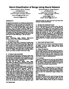
however introduce noise at the same time and result in reduced performance (Chakrabarti, Dom, and Indyk 1998; Myaeng and Lee 2000). Other approaches incorporate the labels of its neighbours. For instance, the Iterative Classification Approach (ICA) integrates the label distribution of neighbouring vertices to assist classification (Lu and Getoor 2003) and the Label Propagation approach (LP) fine-tunes predictions of the vertex using the labels of its neighbouring vertices (Wang and Zhang 2008). However, labels of neighbouring vertices are not representative enough for learning sophisticated relationships of vertices, while using their attributes directly would involve noise. We thus need an approach that is capable of capturing information from neighbouring vertices, while in the mean time reducing noise of attributes. Utilizing representations learned from neural networks instead of neighbouring attributes or labels is one of the possible approaches (Schmidhuber 2015). As graphs normally provide rich structural information, we exploit the neural networks with sufficient complexity for capturing such structures. Recurrent neural networks were developed to utilize sequence structures by processing input in order, in which the representation of the previous node is used to generate the representation of the current node. Recursive neural networks exploit representation learning on tree structures. Both of the approaches achieve success in learning representation of data with implicit structures which indicate the order of processing vertices (Tang, Qin, and Liu 2015; Tai, Socher, and Manning 2015). Following these work, we explore the possibility of integrating graph structures into recursive neural network. However, graph structures, especially cyclic graphs, do not provide such an processing order. In this paper, we propose a graph-based recursive neural network (GRNN), which allows us to transform graph structures to tree structures and use recursive neural networks to learn representations for the vertices to classify. This framework consists of two main components, as illustrated in Figure 1: 1. Tree construction: For each vertex to classify vt , we generate a search tree rooted at vt . Starting from vt , we add its neighbouring vertices into the tree layer by layer. 2. Recursive neural network construction: We build a recursive neural network for the constructed tree, by aug-

Figure 1: Main components of the Graph-based Recursive Neural Network framework (GRNN): 1) constructing a tree from the vertex to classify (vertex 1); 2) building a recursive neural network on the tree.

menting each vertex with one recursive neural unit. The inputs of each vertex are its features and hidden states of its child vertices. The output of a vertex is its hidden states. Our main contributions are: (1) We introduce recursive neural networks to solve the collective vertex classification problem. (2) We propose a method that can transfer vertices for classification to a locally constructed tree. Based on the tree, recursive neural network can extract representations for target vertices. (3) Our experimental results show that the proposed approach outperforms several baseline methods. Particularly, we demonstrate that including information from neighbouring vertices can improve performance of classification.

Related Work There has been a growing trend to represent data using graphs (Angles and Gutierrez 2008). Discovering knowledge from graphs becomes an exciting research area, such as vertex classification (London and Getoor 2014) and graph classification (Niepert, Ahmed, and Kutzkov 2016). Graph classification analyzes the properties of the graph as a whole, while vertex classification focuses on predicting labels of vertices in the graph. In this paper, we discuss the problem of vertex classification. The main-stream approaches for vertex classification are collective vertex classification (Lu and Getoor 2003) which classify vertices using information provided by neighbouring vertices. Iterative classification approach (Lu and Getoor 2003) models neighbours’ label distribution as link features to facilitate classification. Label propagation approach (Wang and Zhang 2008) assigns a probabilistic label for each vertex and then fine-tunes the probability using graph structure. However, labels of neighbouring vertices are not representative enough to include all useful information. Some researchers tried to introduce attributes from neighbouring vertices to improve classification performance. Nevertheless, as reported in (Chakrabarti, Dom, and Indyk 1998; Myaeng and Lee 2000), naively incorporating these features may reduce the performance of classification, when original features of neighbouring vertices are too noisy. Recently, some researchers analysed graphs using deep

neural network technologies. Deepwalk (Perozzi, Al-Rfou, and Skiena 2014) is an unsupervised learning algorithm to learn vertex embeddings using link structure, while content of each vertex is not considered. Convolutional neural network for graphs (Niepert, Ahmed, and Kutzkov 2016) learns feature representations for the graphs as a whole. Recurrent neural collective classification (Monner and Reggia 2013) encodes neighbouring vertices via a recurrent neural network, which is hard to capture the information from vertices that are more than several steps away. Recursive neural networks (RNN) are a series of models that deal with tree-structured information. RNN has been implemented in natural scenes parsing (Socher et al. 2011) and tree-structured sentence representation learning (Tai, Socher, and Manning 2015). Under this framework, representations can be learned from both input features and representations of child nodes. Graph structures are more widely used and more complicated than tree or sequence structures. Due to the lack of notable order for processing vertices in a graph, few studies have investigated the vertex classification problem using recursive neural network techniques. The graph-based recursive neural network framework proposed in this paper can generate the processing order for neural network according to the vertex to classify and the local graph structure.

Graph-based Recursive Neural Networks In this section, we present the framework of Graph-based Recursive Neural Networks (GRNN). A graph G = (V, E) consists of a set of vertices V = {v1 , v2 , . . . , vN } and a set of edges E ⊆ V × V . Graphs may contain cycles, where a cycle is a path from a vertex back to itself. Let X = {x1 , x2 , · · · , xN } be a set of feature vectors, where each xi ∈ X is associated with a vertex vi ∈ V , L be a set of labels, and vt ∈ V be a vertex to be classified, called target vertex. Then, the collective vertex classification problem is to predict the label yt of vt , such that yˆt = arg max Pθ (yt |vt , G, X ) yt ∈L

using a recursive neural network with parameters θ.

(1)

Algorithm 1 Tree Construction Algorithm Require: Graph G, Target vertex vt , Tree depth d Ensure: Tree T = (VT , ET ) 1. Let Q be a queue 2. VT = {vt }, ET = ∅ 3. Q.push(vt ) 4. while Q is not empty do 5. v = Q.pop() 6. if T .depth(v) ≤ d then 7. for w in G.outgoingVertices(v) do 8. // add w to T as child of v 9. VT = VT ∪ {w} 10. ET = ET ∪ {(v, w)} 11. Q.push(w) 12. end for 13. end if 14. end while 15. return T

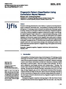
Tree Construction In a neural network, neurons are arranged in layers and different layers are processed following a predefined order. For example, recurrent neural networks process inputs in sequential order and recursive neural networks deal with treestructures in a bottom-up manner. However, graphs, particularly cyclic graphs, do not have an explicit order. How to construct an ordered structure from a graph is challenging. Given a graph G = (V, E), a target vertex vt ∈ V and tree depth d ∈ N, we can construct a tree T = (VT , ET ) rooted at vt using breadth-first-search, where VT is a vertex set, ET is an edge set, and (v, w) ∈ ET means an edge from parent vertex v to child vertex w. The depth of a vertex v in T is the length of the path from vt to v, denoted as T .depth(v). The depth of a tree is maximum depth of vertices in T . We use G.outgoingVertices(v) to denote a set of outgoing vertices from v, i.e. {w|(v, w) ∈ G}. The tree construction algorithm is described in Algorithm 1. Firstly, a first-in-first-out queue (Q) is initialized with vt (lines 1-3). The algorithm iteratively check the vertices in Q. If there is a vertex whose depth is less than d, we pop it out from Q (line 6), add all its neighbouring vertices in G as its children in T and push them to the end of Q (lines 9-11). In general, there are two approaches to deal with cycles in a graph. One is to remove vertices that have been visited, and the other is to keep duplicate vertices. Fig 2.a describes an example of a graph with a cycle between v1 and v2 . Let us start with the target vertex v1 . In the first approach, there will be no child vertex for v2 , since v1 is already visited. The corresponding tree is shown in Fig 2.b. In the second approach, we will add v1 as a child vertex to v2 iteratively and terminate after certain steps. The corresponding tree is illustrated in Fig 2.c. When generating the representation of a vertex, say v2 , any information from its neighbours may help. We thus include v1 as a child vertex of v2 . In this paper, we use the second manner for tree construction.

Figure 2: (a) A graph with a cycle; (b) A tree constructed without duplicate vertices; (c) A tree constructed with duplicate vertices.

Recursive Neural Network Construction Now we construct a recursive neural unit (RNU) for each vertex vk ∈ T . Each RNU takes a feature vector xk and hidden states of its child vertices as input. We explore two kinds of recursive neural units which are discussed in (Socher et al. 2011; Tai, Socher, and Manning 2015). Naive Recursive Neural Unit (NRNU) Each NRNU for a vertex vk ∈ T takes a feature vector xk and the aggregation of the hidden states from all children of vk . The transition equations of NRNU are given as follows: fk = h

max {hr }

(2)

vr ∈C(vk )

fk + b(h) ) hk = tanh(W (h) xk + U (h) h

(3) (h)

where C(vk ) is the set of child vertices of vk , W and U (h) are weight matrix, and b(h) is the bias. The generated hidden state hk of vk is related to the input vector xk and fk . Different from summing up all aggregated hidden state h hidden states as in (Tai, Socher, and Manning 2015), we use fk (see Eq 2). This is because, in real-life max pooling for h situations, the number of neighbours for a vertex can be very large and some of them are irrelevant for the vertex to classify (Zhang et al. 2013). We use G-NRNN to refer to the graph-based naive recursive neural network which incorporates NRNU as recursive neural units. Long Short-Term Memory Unit (LSTMU) LSTMU is one variation on RNU, which can handle the long term dependency problem by introducing memory cells and gated units (Hochreiter and Schmidhuber 1997). LSTMU is composed of an input gate ik , a forget gate fk , an output gate ok , a memory cell ck and a hidden state hk . The transition equations of LSTMU are given as follows: fk = h

max {hr }

(4)

vr ∈C(vk )

fk + b(i) ) ik = σ(W (i) xk + U (i) h

(5)

fkr = σ(W (f ) xk + U (f ) hr + b(f ) )

(6)

ok = σ(W

(o)

xk +

fk U (o) h

+b

(o)

)

fk + b(u) ) uk = tanh(W (u) xk + U (u) h

(7) (8)

ck = ik uk +

X

fkr cr

(9)

vr ∈C(vk )

hk = ok tanh(ck )

(10)

where C(vk ) is the set of child vertices of vk , vr ∈ C(vk ), xk is corresponding feature vector of the child vertex vk , is element-wise multiplication and σ is sigmoid function, W (∗) and U (∗) are weight matrices, and b(∗) are the biases. fk is a vector aggregated from the hidden states of the child h vertices. We use G-LSTM to refer to the graph-based long short-term memory network which incorporates LSTMU as recursive neural units. After constructing GRNN, we calculate the hidden states of all vertices in T from leaves to root, then we use a softmax classifier to predict label yt of the target vertex vt using its hidden states ht (see Eq 11). Pθ (yt |vt , G, X ) = sof tmax(W (s) ht + b(s) ) yˆt = arg max Pθ (yt |vt , G, X ) yt ∈L

(11) (12)

PN Cross-entropy J(θ) = − N1 t=1 log Pθ (yt |vt , G, X ) is used as cost function, where N is the number of vertices in a training set.

Experimental Setup To verify the effectiveness of our approach, we have conducted experiments on four datasets and compared our approach with three baseline methods. We will describe the datasets, baseline methods, and experimental settings.

Datasets We have tested our approach on four real-world network datasets. • Cora (McCallum et al. 2000) is a citation network dataset which is composed of 2708 scientific publications and 5429 citations between publications. All publications are classified into seven classes: Rule Learning (RU), Genetic Algorithms (GE), Reinforcement Learning (RE), Neural Networks (NE), Probabilistic Methods (PR), Case Based (CA) and Theory (TH). • Citeseer (Giles, Bollacker, and Lawrence 1998) is another citation network dataset which is larger than Cora. Citeseer is composed of 3312 scientific publications and 4723 citations. All publications are classified into six classes: Agents, AI, DB, IR, ML and HCI. • WebKB (Craven et al. 1998) is a website network collected from four computer science departments in different universities which consists of 877 web pages, 1608 hyper-links between web pages. All websites are classified into five classes: faculty, students, project, course and other. • WebKB-sim is a network dataset which is generated from WebKB based on the cosine similarity between each vertex and its top 3 similar vertices according to their feature vectors (Baeza-Yates, Ribeiro-Neto, and others 1999). We use same feature vectors as the ones in WebKB. This

dataset is used to demonstrate the effectiveness of our framework on datasets which may not have explicit relationship represented as edges between vertices, but can be treated as graphs whose edges are based on some metrics such as similarity of vertices. We use abstracts of publications in Cora and Citeseer, and contents of web pages in WebKB to generate features of vertices. For the above datasets, all words are stemmed first, then stop words and words with document frequency less than 10 are discarded. A dictionary is generated by including all these words. We have 1433, 3793, and 1703 for Cora, Citeseer and WebKB, respectively. Each vertex is represented by a bag-of-words vector where each dimension indicates absence or occurrence of a word in the dictionary of the corresponding dataset1 .

Baseline Methods We have implemented the following three baseline methods: • Logistic Regression (LR) (Hosmer Jr and Lemeshow 2004) predicts the label of a vertex using its own attributes through a logistic regression model. • Iterative classification approach (ICA) (Lu and Getoor 2003; London and Getoor 2014) utilizes the combination of link structure and vertex features as input of a statistical machine learning model. We use two variants of ICA: ICA-binary uses the occurrence of labels of neighbouring vertices, ICA-count uses the frequency of labels of neighbouring vertices. • Label propagation (LP) (Wang and Zhang 2008; London and Getoor 2014) uses a statistical machine learning to give a label probability for each vertex, then propagates the label probability to all its neighbours. The propagation steps are repeated until all label probabilities converge. To make experiments consistent, logistic regression is used for all statistical machine learning components in ICA and LP. We run 5 iterations for each ICA experiment and 20 iterations for each LP experiment2 .

Experimental Settings In our experiments, we split each dataset into two parts: training set and testing set, with different proportions (70% to 95% for training). For each proportion setting, we randomly generate 5 pairs of training and testing sets. For each experiment on a pair of training and testing sets, we run 10 epochs on the training set and record the highest Micro-F1 score (Baeza-Yates, Ribeiro-Neto, and others 1999) on the testing set. Then we report the averaged results from the experiments with the same proportion setting. According to preliminary experiments, the learning rate is set to 0.1 for LR, ICA and LP and 0.01 for all GRNN models. We empirically set number of hidden states to 200 for all GRNN models. Adagrad (Duchi, Hazan, and Singer 2011) is used as the optimization method in our experiments. 1

Cora, Citeseer and WebKB can be downloaded from LINQS. We will publish WebKB-sim along with our code. 2 According to our preliminary experiments, LP converges slower than ICA.

(a) Cora G-NRNN

Micro F1-score (%)

(b) Citeseer G-NRNN

G-NRNN_d0 G-NRNN_d1 G-NRNN_d2

86

(d) WebKB-sim G-NRNN

90

90

76

88

88

82

74

86

86

80

72

84

84

78

70

82

82

84

76

68

80

80

0.70 0.75 0.80 0.85 0.90 0.95

0.70 0.75 0.80 0.85 0.90 0.95

0.70 0.75 0.80 0.85 0.90 0.95

(e) Cora G-LSTM

(f) Citeseer G-LSTM

(g) WebKB G-LSTM

G-LSTM_d0 G-LSTM_d1 G-LSTM_d2

86

Micro F1-score (%)

(c) WebKB G-NRNN

78

84

0.70 0.75 0.80 0.85 0.90 0.95

(h) WebKB-sim G-LSTM

78

90

90

76

88

88

82

74

86

86

80

72

84

84

78

70

82

82

76

68 0.70 0.75 0.80 0.85 0.90 0.95

80 0.70 0.75 0.80 0.85 0.90 0.95

Training Proportion

80 0.70 0.75 0.80 0.85 0.90 0.95

Training Proportion

0.70 0.75 0.80 0.85 0.90 0.95

Training Proportion

Training Proportion

Figure 3: Comparison of G-NRNN and G-LSTM on four datasets: (a) Cora G-NRNN, (b) Citeseer G-NRNN, (c) WebKB G-NRNN, (d) WebKB-sim G-NRNN (e) Cora G-LSTM, (f) Citeseer G-LSTM, (g) WebKB G-LSTM and (h) WebKB-sim G-LSTM.

LR ICA-binary ICA-count

Micro F1-score (%)

86

(a) Cora

(b) Citeseer

LP G-NRNN_d2 G-LSTM_d2

(c) WebKB

(d) WebKB-sim

78

90

90

84

76

88

88

82

74

86

86

80

72

84

84

78

70

82

82

76

68 0.70

0.75

0.80

0.85

0.90

Training Proportion

0.95

80 0.70

0.75

0.80

0.85

0.90

Training Proportion

0.95

80 0.70

0.75

0.80

0.85

0.90

Training Proportion

0.95

0.70

0.75

0.80

0.85

0.90

Training Proportion

0.95

Figure 4: Comparison of G-LSTM with LR, LP and ICA on four datasets: (a) Cora, (b) Citeseer, (c) WebKB and (d) WebKB-sim.

Results and Discussion Model and Parameter Selection Figure 3 illustrates the performance of G-NRNN and GLSTM on four datasets. We use G-NRNN di and GLSTM di to refer to G-NRNN and G-LSTM over trees of depth i, respectively, where i = 0, 1, 2. For the experiments on G-NRNN and G-LSTM over trees of different steps, d1 and d2 outperform d0 in most cases3 . Particularly, the experiments with d1 and d2 perform better with more than 2% improvement than d0 on Cora, and d1 and d2 enjoy a consistent improvement over d0 on Citeseer and WebKB-sim. This performance difference is also obvious in WebKB, when the training proportion is larger than 85%. These mean that introducing neighbouring vertices can improve the performance of classification and more neighbouring information can be obtained by increasing the depth 3

When d = 0, each constructed tree contains only one vertex.

of trees. Using same RNU setting, d2 outperforms d1 in most experiments on Cora, Citeseer and WebKB-sim. However, for WebKB, d2 does not always outperforms d1. That is to say, introducing more layers of vertices may help improving the performance, while the choice of the best tree depth depends on applications.

Table 1: Micro-F1 score (%) of G-LSTM model with different pooling strategies on Cora, Citeseer, WebKB and WebKB-sim. Method

G-LSTM d1

G-LSTM d2

Pooling Strategy

Cora

Citeseer

sum mean max sum mean max

83.05 84.18 83.83 84.03 84.47 84.72

74.81 74.77 74.89 75.05 75.33 75.45

Datasets WebKB 86.21 86.21 87.12 85.61 86.21 86.06

WebKB-sim 87.42 87.58 87.42 87.42 87.42 87.73

Figure 5: Distribution of label co-occurrence for Cora, Citeseer, WebKB and WebKB-sim, where d = 1, 2.

In Table 1, we compare three different pooling strategies used in G-LSTM4 , sum, mean and max pooling. We use 85% for training for all datasets here. In general, mean and max outperform sum which is used in (Tai, Socher, and Manning 2015). This is probably because, the number of neighbours for a vertex can be very large and summing them up can make e h large for some extreme cases. max slightly outperforms mean in our experiments, which is probably due to max pooling can select the most influential information of child vertices which filters out noise to some extend.

Baseline Comparison We compare our approach with the baseline methods on four network datasets. As our models with d2 provide better performance, we choose G-NRNN d2 and G-LSTM d2 as representative models. In Figure 4.a and Figure 4.b, we compare our approach with the baseline methods on two citation networks, Cora and Citeseer. The collective vertex classification approaches, i.e. LP, ICA, G-NRNN and G-LSTM, largely outperform LR which only uses attributes of the target vertex. Both G-NRNN d2 and G-LSTM d2 consistently outperform all baseline methods on the citation networks, which indicates the effectiveness of our approach. In Figure 4.c and Figure 4.d, we compare our approach with the baseline methods on WebKB and WebKB-sim. For WebKB, our method obtains competitive results in comparison with ICA. LP works worse than LR on WebKB, where Micro-F1 score is less than 0.7. For this reason, it is not presented in Figure 4.c, and we will discuss this in detail in the next subsection. For WebKB-sim, our approaches consistently outperform all baseline methods, and G-LSTM d2 outperforms GNRNN d1 when the training proportion is larger than 80%. In general, G-LSTM d2 outperforms G-NRNN d2. This 4 As G-NRNN gives similar results, we only illustrate results for G-LSTM here

is likely due to the LSTMU’s capability of memorizing information using memory cells. G-LSTM can thus better capture correlations between representations with long dependencies (Hochreiter and Schmidhuber 1997).

Dataset Comparison To analyse co-occurrence of neighbouring labels, we compute the transition probability from target vertices to their neighbouring vertices. We first calculate the label cod occurrence matrix M d , where Mi,j indicates co-occurred times of labels li of target vertices vi and labels lj of d-step away vertices vj . Then we obtain probability maPa transition d d d trix T d , where Ti,j = Mi,j /( k Mi,k ). The heat maps of T d on four datasets are demonstrated in Figure 5. For Cora and Citeseer, neighbouring vertices tend to share same labels. When d increases to 2, labels are still tightly correlated. That is probably why all ICA, LP G-NRNN and G-LSTM work well on Cora and Citeseer. In this situation, GRNN integrates features of d-step away vertices which may directly help classify a target vertex. For WebKB, correlation of labels is not clear, some label can be strongly related to more than two labels, e.g. students connects to course, project and student. Introducing vertices which are more steps away makes the correlation even worse for WebKB, e.g.all labels are most related to student. In this situation, LP totally fails, while ICA can learn the correlation of labels that are not same, i.e. student may relate to course instead of student itself. For this dataset, GRNN still achieves competitive results with the best baseline approach. For WebKB-sim, although student is still the label with highest frequency, the correlation between labels is clearer than WebKB, i.e. project relates to project and student. That is probably the reason why, the performance of our approach is good on WebKB-sim for both settings and G-LSTM d2 achieves better results than G-NRNN d2 when the training proportion is larger.

Conclusions and Future work In this paper, we have presented a graph-based recursive neural network framework(GRNN) for vertex classification on graphs. We have compared two recursive units, NRNU and LSTMU within this framework. It turns out that LSTMU works better than NRNU on most experiments. Finally, the performance of our proposed methods outperformed several state-of-the-art statistical machine learning based methods. In the future, we intend to extend this work in several directions. We aim to apply GRNN to large scale graphs. We also aim to improve the efficiency of GRNN and conduct time complexity analysis.

References Angles, R., and Gutierrez, C. 2008. Survey of graph database models. ACM Computing Surveys (CSUR) 40(1):1. Baeza-Yates, R.; Ribeiro-Neto, B.; et al. 1999. Modern information retrieval, volume 463. ACM press New York. Chakrabarti, S.; Dom, B.; and Indyk, P. 1998. Enhanced hypertext categorization using hyperlinks. In ACM SIGMOD Record, volume 27, 307–318. ACM. Craven, M.; DiPasquo, D.; Freitag, D.; and McCallum, A. 1998. Learning to extract symbolic knowledge from the world wide web. In Proceedings of the 15th National Conference on Artificial Intelligence, 509–516. American Association for Artificial Intelligence. Duchi, J.; Hazan, E.; and Singer, Y. 2011. Adaptive subgradient methods for online learning and stochastic optimization. Journal of Machine Learning Research 12(Jul):2121– 2159. Giles, C. L.; Bollacker, K. D.; and Lawrence, S. 1998. Citeseer: An automatic citation indexing system. In Proceedings of the 3rd ACM conference on Digital libraries, 89–98. ACM. Hochreiter, S., and Schmidhuber, J. 1997. Long short-term memory. Neural computation 9(8):1735–1780. Hosmer Jr, D. W., and Lemeshow, S. 2004. Applied logistic regression. John Wiley & Sons. London, B., and Getoor, L. 2014. Collective classification of network data. Data Classification: Algorithms and Applications 399. Lu, Q., and Getoor, L. 2003. Link-based classification. In Proceedings of the 20th International Conference on Machine Learning, volume 3, 496–503. McCallum, A. K.; Nigam, K.; Rennie, J.; and Seymore, K. 2000. Automating the construction of internet portals with machine learning. Information Retrieval 3(2):127–163. Monner, D. D., and Reggia, J. A. 2013. Recurrent neural collective classification. IEEE transactions on neural networks and learning systems 24(12):1932–1943. Myaeng, S. H., and Lee, M.-h. 2000. A practical hypertext categorization method using links and incrementally available class information. In Proceedings of the 23rd ACM International Conference on Research and Development in Information Retrieval. ACM.

Niepert, M.; Ahmed, M.; and Kutzkov, K. 2016. Learning convolutional neural networks for graphs. In Proceedings of the 33rd International Conference on Machine Learning. Perozzi, B.; Al-Rfou, R.; and Skiena, S. 2014. Deepwalk: Online learning of social representations. In Proceedings of the 20th ACM SIGKDD International Conference on Knowledge Discovery and Data Mining, 701–710. ACM. Schmidhuber, J. 2015. Deep learning in neural networks: An overview. Neural Networks 61:85–117. Socher, R.; Lin, C. C.; Manning, C.; and Ng, A. Y. 2011. Parsing natural scenes and natural language with recursive neural networks. In Proceedings of the 28th International Conference on Machine Learning, 129–136. Tai, K. S.; Socher, R.; and Manning, C. D. 2015. Improved semantic representations from tree-structured long short-term memory networks. In Proceedings of the 53rd Annual Meeting of the Association for Computational Linguistic. ACL. Tang, J.; Chang, S.; Aggarwal, C.; and Liu, H. 2015. Negative link prediction in social media. In Proceedings of the Eighth ACM International Conference on Web Search and Data Mining, 87–96. ACM. Tang, D.; Qin, B.; and Liu, T. 2015. Document modeling with gated recurrent neural network for sentiment classification. In Proceedings of the 2015 Conference on Empirical Methods in Natural Language Processing, 1422–1432. Wang, F., and Zhang, C. 2008. Label propagation through linear neighborhoods. IEEE Transactions on Knowledge and Data Engineering 20(1):55–67. Zhang, J.; Liu, B.; Tang, J.; Chen, T.; and Li, J. 2013. Social influence locality for modeling retweeting behaviors. In Proceeding of the 23rd International Joint Conference on Artificial Intelligence, volume 13, 2761–2767. Citeseer.