Neural Network Design for. Switching Network Control. Thesis by. Timothy X
Brown. In Partial Fulfillment of the Requirements for the Degree of. Doctor of ...
Neural Network Design for Switching Network Control Thesis by Timothy X Brown In Partial Fulfillment of the Requirements for the Degree of Doctor of Philosophy
California Institute of Technology Pasadena, California 1991 (Submitted June 29, 1990)
ii
c
1991 Timothy X Brown All rights reserved
iii
Acknowledgements Many more people than the one named on the cover influenced the content of this thesis and even the fact that you are reading this now. Thanks goes to each of these individuals. First and foremost honor goes to my advisor Edward C. Posner whose knowledge, seemingly endless in breadth, and insights appear throughout this thesis. He also suggested and guided the development of the thesis topic. Many fellow graduate students added ideas and were sounding boards to my own ideas, as well as being friends. These include Kathleen Kramer, Zorana Popovi´c, Ivan Onyszchuk, Gabriel Rabeiz, Rajaram Ramesh, John Miller, and Kumar Sivarajan. Special thanks goes to Dr. Kuo-Hui Liu of Pacific Bell. He introduced me to the ATM switching problem and suggested several avenues of approach. Pacific Bell provided generous grants to the EE systems group that not only supported me throughout my research at Caltech, but also provided extensive computing facilities. On a more personal level I must thank: my parents for their support; my brother and sister for spurring me on to higher education; and my grandparents who each in their own way positively influenced my academic career. To my wife I reserve my greatest gratitude. All my experiences at Caltech are intimately intertwined with her.
iv
Abstract A neural network is a highly interconnected set of simple processors. The many connections allow information to travel rapidly through the network, and due to their simplicity, many processors in one network are feasible. Together these properties imply that we can build efficient massively parallel machines using neural networks. The primary problem is how do we specify the interconnections in a neural network. The various approaches developed so far such as outer product, learning algorithm, or energy function suffer from the following deficiencies: long training/specification times; not guaranteed to work on all inputs; requires full connectivity. Alternatively we discuss methods of using the topology and constraints of the problems themselves to design the topology and connections of the neural solution. We define several useful circuits—generalizations of the Winner-Take-All circuit— that allows us to incorporate constraints using feedback in a controlled manner. These circuits are proven to be stable, and to only converge on valid states. We use the Hopfield electronic model since this is close to an actual implementation. We also discuss methods for incorporating these circuits into larger systems, neural and nonneural. By exploiting regularities in our definition, we can construct efficient networks. To demonstrate the methods, we look to three problems from communications. We first discuss two applications to problems from circuit switching; finding routes in large multistage switches, and the call rearrangement problem. These show both, how we can use many neurons to build massively parallel machines, and how the Winner-Take-All circuits can simplify our designs. Next we develop a solution to the contention arbitration problem of high-speed packet switches. We define a useful class of switching networks and then design a neural network to solve the contention arbitration problem for this class. Various aspects of the neural network/switch system are analyzed to measure the queueing performance of this method. Using the basic design, a feasible architecture for a large (1024-input) ATM packet switch is presented. Using the massive parallelism of neural networks, we can consider algorithms that were previously computationally
v unattainable. These now viable algorithms lead us to new perspectives on switch design.
Contents 1 Introduction:
1
1.1 What is a Neural Network and What Will We Show? . . . . . . . . .
1
1.2 Neural Networks and Parallel Machines . . . . . . . . . . . . . . . . .
2
1.3 Neural Networks . . . . . . . . . . . . . . . . . . . . . . . . . . . . .
4
1.4 Designing Neural Networks . . . . . . . . . . . . . . . . . . . . . . . .
5
1.5 Saying What We Said . . . . . . . . . . . . . . . . . . . . . . . . . .
7
1.6 Thesis Outline . . . . . . . . . . . . . . . . . . . . . . . . . . . . . . .
8
2 Designing with Neural Networks
11
2.1 Introduction . . . . . . . . . . . . . . . . . . . . . . . . . . . . . . . .
11
2.2 Neural Network Model . . . . . . . . . . . . . . . . . . . . . . . . . .
11
2.3 The Winner-Take-All Circuit . . . . . . . . . . . . . . . . . . . . . . .
14
2.4 The Multiple Overlapping Winner-Take-All Circuit . . . . . . . . . .
18
2.5 The Multiple Overlapping K-Winner-Take-All Circuit . . . . . . . . .
20
2.6 Neuron Gain . . . . . . . . . . . . . . . . . . . . . . . . . . . . . . . .
22
2.7 Designing with Winner-Take-All Circuits . . . . . . . . . . . . . . . .
25
2.8 Conclusions . . . . . . . . . . . . . . . . . . . . . . . . . . . . . . . .
26
2.A Winner-Take-All Dynamics . . . . . . . . . . . . . . . . . . . . . . . .
27
3 Controlling Circuit Switching Networks
31
3.1 Introduction . . . . . . . . . . . . . . . . . . . . . . . . . . . . . . . .
31
3.2 Background on Switches . . . . . . . . . . . . . . . . . . . . . . . . .
31
3.3 Large Multistage Switching Networks . . . . . . . . . . . . . . . . . .
34
vi
vii 3.4
Finding Routes using Neural Networks . . . . . . . . . . . . . . . . .
37
3.5
Rearrangeable Switches . . . . . . . . . . . . . . . . . . . . . . . . . .
39
3.6
The Neural Network Solution to the Rearrangement Problem . . . . .
44
3.7
Conclusion . . . . . . . . . . . . . . . . . . . . . . . . . . . . . . . . .
57
4 Banyan Network Controller
60
4.1
Introduction . . . . . . . . . . . . . . . . . . . . . . . . . . . . . . . .
60
4.2
ATM switching networks . . . . . . . . . . . . . . . . . . . . . . . . .
60
4.3
Banyan Networks . . . . . . . . . . . . . . . . . . . . . . . . . . . . .
63
4.4
Blocking Constraints and Deterministic Switches . . . . . . . . . . . .
65
4.5
Queueing . . . . . . . . . . . . . . . . . . . . . . . . . . . . . . . . .
67
4.6
The Neural Network Solution . . . . . . . . . . . . . . . . . . . . . .
72
4.7
Network Prompting . . . . . . . . . . . . . . . . . . . . . . . . . . . .
73
4.8
Simulation Results . . . . . . . . . . . . . . . . . . . . . . . . . . . .
75
4.9
Implementation Considerations . . . . . . . . . . . . . . . . . . . . .
83
4.10 Buffered Memory Switches and Large Switch Designs . . . . . . . . .
87
4.11 Conclusions . . . . . . . . . . . . . . . . . . . . . . . . . . . . . . . .
90
4.A Estimating the Tails . . . . . . . . . . . . . . . . . . . . . . . . . . .
91
5 Epilogue
98
List of Figures 1.1 Loss in computational efficiency. . . . . . . . . . . . . . . . . . . . . .
3
1.2 Solution to the parity problem. . . . . . . . . . . . . . . . . . . . . .
7
2.1 The electronic neural model. . . . . . . . . . . . . . . . . . . . . . . .
12
2.2 Winner-Take-All mutual inhibition circuit. . . . . . . . . . . . . . . .
15
2.3 The Multiple Overlapping Winner-Take-All concept. . . . . . . . . . .
18
2.4 A set matrix showing the equivalence of the threshold definitions. . .
19
3.1 The N × N crossbar switch concept. . . . . . . . . . . . . . . . . . .
32
3.2 A general three-stage switch. . . . . . . . . . . . . . . . . . . . . . . .
34
3.3 Multistage switch. . . . . . . . . . . . . . . . . . . . . . . . . . . . . .
35
3.4 Multistage switch with five calls already put up. . . . . . . . . . . . .
36
3.5 Neural network for switch path search. . . . . . . . . . . . . . . . . .
38
3.6 Neural network searching for a path. . . . . . . . . . . . . . . . . . .
40
3.7 Paull matrix. . . . . . . . . . . . . . . . . . . . . . . . . . . . . . . .
42
3.8 A blocked call request at (2, 3). . . . . . . . . . . . . . . . . . . . . .
43
3.9 Unblocking rearrangement for call request. . . . . . . . . . . . . . . .
44
3.10 Three-dimensional neuron grid. . . . . . . . . . . . . . . . . . . . . .
46
3.11 Additional memory neuron. . . . . . . . . . . . . . . . . . . . . . . .
50
3.12 Neural network solving blocking situation. . . . . . . . . . . . . . . .
52
3.13 Additional circuitry to force the network to follow Paull’s algorithm. .
53
3.14 Solving the rearrangement problem for n = 3. . . . . . . . . . . . . .
55
4.1
An 8 × 8 Banyan switching network. . . . . . . . . . . . . . . . . . .
64
4.2
Equivalence classes. . . . . . . . . . . . . . . . . . . . . . . . . . . . .
68
viii
ix 4.3
The queueing model. . . . . . . . . . . . . . . . . . . . . . . . . . . .
69
4.4
Mapping from the queue state to a cell matrix. . . . . . . . . . . . . .
71
4.5
Demonstration of smoothing.
. . . . . . . . . . . . . . . . . . . . . .
77
4.6
Average queue size vs. average number of arrivals (Bernoulli). . . . .
79
4.7
Average queue size vs. average number of arrivals (batch). . . . . . .
80
4.8
Performance range. . . . . . . . . . . . . . . . . . . . . . . . . . . . .
81
4.9
Control architecture comparison. . . . . . . . . . . . . . . . . . . . .
82
4.10 A schematic of the queue architecture for one of the input queues. . .
85
4.11 The buffered-memory Banyan hybrid switch. . . . . . . . . . . . . . .
88
4.12 A sample of a queue size distribution. . . . . . . . . . . . . . . . . . .
92
x
List of Tables 2.1 Comparison of necessary neuron gains . . . . . . . . . . . . . . . . . .
24
3.1 Tally of the neural rearranger size.
. . . . . . . . . . . . . . . . . . .
56
4.1 Buffer size estimates. . . . . . . . . . . . . . . . . . . . . . . . . . . .
84
4.2 Buffer size necessary for the hybrid switch. . . . . . . . . . . . . . . .
90
1
Chapter 1 Introduction: Has parallel computing failed us again? —W. L. Miranker [1]
1.1
What is a Neural Network and What Will We Show?
Neural networks are a class of systems that have many simple processors —“neurons”— that are highly interconnected. The function of each neuron is simple, and the behavior is determined predominantly by the set of interconnections. Thus, a neural network is a special form of parallel computer. Although a major impetus for using neural networks is that they may be able to “learn” the solution to the problem that they are to solve, we argue that another perhaps stronger impetus is that they provide a framework for designing massively parallel machines. As a step in this direction, we develop techniques which will aid us in our designs. The highly interconnected architecture of switching networks suggests similarities to neural networks, and indeed, we present three applications in switching in which neural networks can solve the problems efficiently. The first two problems come from circuit switching: finding routes through large multistage switches and calculating a rearrangement that allows a new call to be placed through a rearrangeable switch. In this latter problem we show that a computational advantage can be gained by using nonuniform time delays in the network. The last application is to high-speed
2 interconnection networks, of relevance to packet switching. Using the computational speed of many neural processors working in parallel, we are able to resolve contention for paths through the network in the necessary time. We analyze this problem in detail to show the applicability of neural systems to real applications.
1.2
Neural Networks and Parallel Machines
For applications requiring computational speed beyond what a single processor is capable of, increasing the number of processors can decrease the computation time. Standard parallel computing models are all fundamentally equivalent to the Turing model of computation. While, in principle, the programming of the multiple nodes is a straightforward extension of the programming of a single node, unfortunately, complications arise since the processors must spend time communicating intermediate results and waiting for other processors to send needed data. The programming and even the way that the multiple processors must be connected so that the machine isn’t bogged down in this interprocessor-communication and scheduling overhead is not so well understood. As a result, the increase in speed as a function of the number of processors is significantly sublinear. We illustrate this phenomenon using data from reference [2]. The time using one processor for a given task is less than N times the time spent with N processors. Putting this in a comparable form, we define: 4
Loss in Efficiency =
N × (time using N processors) − (time using 1 processor) N × (time using N processors)
Figure 1.1 shows examples of the loss in efficiency as a function of the number of processors for some common parallel machines. This was from a performance test that allowed the manufacturers to use the fastest possible algorithm that they could develop to solve a system of 1000 equations and 1000 unknowns. This comparison is interesting because these machines have a variable number of processors. By comparing only within a single architecture, we can control for the differences between machines. The loss in efficiency is significant for
3
Figure 1.1: Loss in computational efficiency. the architectures in the graph. For example, with just seven processors, the Alliant computer spends almost 25% of each processor’s time on this communications overhead. Over the domain of the data given, the loss in efficiency grows linearly with the number of processors. The linear increase in the loss in efficiency implies a decreasing amount of speedup that, if extended, would ultimately lead to an absolute decrease in the computing speed. This does not bode well for systems with many processors. Even if the design and programming problems could be solved, a microprocessor with its associated memory and support components is a complex and relatively expensive computational element, limiting the number of processors. Certainly the idea of 1,000,000 microprocessors in a system does not yet seem feasible. Alternatively one can consider neural networks. While they don’t fit into the von Neumann/Turing framework (although some researchers have been able to formulate special cases within this framework as feedforward threshold-logic circuits), much
4 work has gone into developing their theory. General theorems on their behavior have been derived [3][4]. In digital systems, we typically speak in terms of “0” or “1,” despite the fact that these symbols only represent real valued voltages and currents that exist inside a real system. Furthermore, the logical operation of elements, such as the AND gate or the flip flop, also represents more complex underlying behavior. There exist similar abstractions that simplify the analysis of neural network systems. Thus, we often can treat the neuron as a simple threshold element whose output is either “−1” or “+1.” We will also introduce neural network elements that will allow us to introduce feedback in a controlled manner. Using these elements as building blocks, similar to the use of flip flops, etc., in digital systems, releases us from the details of the underlying dynamics. Because of the simplicity of the individual neurons and because the connections themselves are an integral part of the system’s computation, large neural networks are feasible and useful. Biological neural systems, such as the brains of mammals, show that systems with as many as 1012 neurons are possible. The problem that arises is how to configure a network to solve a particular problem.
1.3
Neural Networks
Before discussing the details of the neural network model that we use, we describe some general principles. The basic unit of an artificial neural network is the neuron. Its function is extremely simple, usually just a threshold function on the weighted sum of its inputs. The functionality of the network is not derived from the operation of the individual neurons, but from the collective properties derived from the many connections between the neurons. The problem in any neural network is to define these connections so that the network operates as desired. There are three issues that arise: • Can we determine these connections in a simple manner? It has been shown theoretically that in general this problem belongs to a class of “hard” problems [5]. This is true even for simple neural architectures [6]. Empirically it is
5 known that the number of iterations needed to converge on a set of connections grows quickly as the size of network grows [7][8]. Because of this, we cannot guarantee that learning algorithms such as “Back-Propagation,” or “The Boltzmann Machine,” will find a working set of connections in a reasonable amount of time. Furthermore, if we must modify the problem (e.g., go to a larger size), does the procedure for specifying the weights have to be repeated all over again. • If we have x neurons, then in general a network may have x2 connections, one from every neuron to every other neuron. Most methods of specifying the connections require such a so-called fully interconnected network. For large networks, this can become prohibitively complex. • Does the set of connections found actually find a valid solution for all possible inputs? Methods proposed in the literature have been shown to work statistically when the number of desired stable states is small compared to the number of neurons [9], or empirically [8] for small problems. These conditions are unreasonable for most applications. For this reason we can never be sure that for the networks found by these methods there isn’t some input that will be problematic.
The method that we propose for the applications in this thesis is to simply design the set of connections for a problem using direct methods, with sub-networks that are already available.
1.4
Designing Neural Networks
This idea is analogous to the work of a digital designer. Given a problem, the designer doesn’t look directly at desired input and output signals and then solder a circuit using transistors, resistors, and other components; rather they analyze what they know about the problem to formulate a solution using the already available AND gates, flip-flops, etc., leading to a circuit design. A good designer will often try to
6 produce a solution to the general class of problems, not just the specific instance that is at hand. Our approach with neural networks will be similar. Given a problem, analysis can yield much information about the problem. We often know the constraints and the direct causes of particular elements in the response. It is therefore to our advantage to incorporate this knowledge into the neural solution. As research continues on neural networks, the number of classes of neural networks which are well understood increases. These can help us to incorporate the knowledge we have about the problem. The fact that a neural network can assume quite arbitrary topologies is extremely useful. The topology of the neural network can be matched to the topology of the problem. This obviates the correspondence between the problem and the neural solution. Finally, since we know the underlying structure which is producing the neural network, we can exploit this structure to simplify the construction. These principles will be very important in guiding us to our design solutions. To introduce some of the basic ideas, consider the infamous (in neural circles) parity check problem: Given N inputs of “−1” or “+1,” output a “+1” if the number of input “1’s” is odd, otherwise output a “−1.” This is often quoted as an unnatural and difficult problem for neural networks to solve [10]. General learning algorithms have great difficulty in finding a solution to the parity check problem. But it is known that there exists a straightforward neural network to solve this for any N ; we present this network below. The way to solve this problem here is to count the number of “+1’s” in the input, and then to see if this number is odd or even. So we first create N neurons numbered 1 through N . We connect neuron i so that it only turns on if there are at least i “+1’s” in the input. We then create an output neuron that uses this regularity to only turn on if the number of “+1’s” is odd. This clearly works. The network is shown in Figure 1.2 [8, p. 334]. Once a solution exist for a class of problems, then as the size of the problem becomes larger, the many processors in the corresponding network can reduce the time of the computation. In the example of the parity problem, all the elements are
7
Figure 1.2: Solution to the parity problem. feedforward, and the output is only two stages from the input, independent of N . This implies—to a first order approximation—that the time to solve the problem is constant for all N . One must be a little careful in the solution, though. First, the number of neurons and connections must not grow too fast with the problem. Second, the time for the network to produce the output must not grow too quickly either. Thus a solution to the parity problem using 2N neurons and connections, or in which the number of stages between the input and the output is N 2 , for example, would not be acceptable. In all of our solutions we will be careful to show that both the component and time complexity is reasonable.
1.5
Saying What We Said
We argue that neural networks are a significant break from conventional parallel computing. Whereas the fundamental problem with conventional parallelism is how to program the multiprocessors; with neural networks it is how to determine the connections between processors. Most current methods assume that the problem
8 is unstructured, unnecessarily ignoring available information. By designing solutions using available information, we can produce efficient general neural solutions to whole classes of problems.
1.6
Thesis Outline
Chapter 2 will present the core analytical results. We present the basic neural model and define three generalizations to the Winner-Take-All neural circuit. Each of these generalizations is shown rigorously to be stable and only converge on stable states. A certain flexibility is incorporated into these designs. We develop methods for utilizing this flexibility for particular applications. By exploiting the regularities in the design, we present methods for significantly reducing the connectivity, while still maintaining identical functionality. Chapters 3 and 4 discuss specific applications of these methods. Chapter 3 contains two applications to problems from circuit switching; finding routes in large multistage switches, and the call rearrangement problem. These will show both, how we can use many neurons to build massively parallel machines, and how the WinnerTake-All circuits can simplify our designs. Chapter 4 is a complete development of an application to high-speed packet switches. We define a useful class of switching networks and then design a neural network to solve the contention arbitration problem for this class. Various aspects of the neural network/switch system are analyzed to measure the queueing performance of this method. Using the basic design, a feasible architecture for a large (1024-input) packet switch is presented.
9
Bibliography [1] Miranker, W. L., Has Parallel Computing Failed Again? A Manifesto for Parallel Computation, EE Systems Seminar presented at Caltech, March 12, 1990. [2] Dongara, J. J., Performance of Various Computers Using Standard Linear Equations Software in a Fortran Environment. Argonne Nat. Lab. Technical Memorandum No. 23, August 13, 1988. [3] Hopfield, J. J., Neurons with Graded Response Have Collective Computational Properties Like Those of Two-State Neurons, Proceedings of the National Academy of Sciences USA, Vol. 81, May 1984, pp. 3088–3092. [4] Marcus, C. M., Westervelt, R. M., Stability of Analog Neural Networks with Delay, Physical Review A, Vol. 39, 1989, pp. 347–359. [5] Judd, J. S., Neural Network Design and the Complexity of Learning, MIT Press, Cambridge, MA, 1990. [6] Blum, A., Rivest, R. L., Training a 3-Node Neural Network is NP-Complete, ed. Touretzky, D. S., Advances in Neural Information Processing Systems I, Morgan Kaufman Pub., San Mateo, CA, 1989, pp. 494–501. [7] Hinton, G. E., Sejnowski, T. J., Learning and Relearning in Boltzmann Machines, ed. Rumelhart, D. E., McClelland, J. L., Parallel Distributed Processing: Explorations in the Microstructure of Cognition. Volume 1: Foundations, MIT Press, Cambridge, MA, 1986, Chapter 7.
10 [8] Rumelhart, D. E., Hinton, G. E., Williams, R. J., Learning Internal Representations by Error Propagation, ed. Rumelhart, D. E., McClelland, J. L., Parallel Distributed Processing: Explorations in the Microstructure of Cognition. Volume 1: Foundations, MIT Press, Cambridge, MA, 1986, Chapter 8. [9] McEliece, R. J., Posner, E. C., Rodemich, E. R., Venkatesh, S. S., The Capacity of the Hopfield Associative Memory, IEEE Transactions on Information Theory, Vol. 33, No. 4, pp. 461–482, Jul. 1987. [10] Minsky, M. L., Papert, S. A., Perceptrons: An Introduction to Computational Geometry, Expanded Edition, MIT Press, Cambridge, MA, 1988, p. 153.
11
Chapter 2 Designing with Neural Networks It could be that the nonlinear nature of inhibitory feedback is the key to building a complex analog processing system with a great deal of gain and time delay, and to keeping the entire mess stable. We will know that we understand these matters only when we can build such a system—and can keep it stable. —Carver A. Mead [1]
2.1
Introduction
In this chapter we will discuss the neural model which will be the starting point of our work. We will then develop a series of increasingly complex neural network classes that will lead us to an understanding of how we can build stable complex analog processing systems that can be applied to specific problems.
2.2
Neural Network Model
We start with the Hopfield continuous model [2], since it is defined in terms of electronic components, and therefore close to an actual implementation. In this model the neurons are high-gain amplifiers that are interconnected through resistors as shown in Figure 2.1 for a four-neuron network. The amplifiers have both positive and negative outputs. A connection from a positive output is known as excitatory, and a connection from a negative output is known as inhibitory. We define W = {wij }, the connection matrix. If Rij is the value of the resistive connection from neuron j to neuron i, then we say that the strength of the connection, |wij |, is 1/Rij . The sign
12
Figure 2.1: The electrical model of a neural network showing topology and details of a neuron.
13 of wij is positive or negative depending on whether the connection is excitatory or inhibitory. Each neuron can have an external input, Ii . A threshold, ti , is subtracted from all the inputs, and the result is the net input to the neuron. In a system of N neurons, given a neuron i, its state variable, ui , is governed by the differential equation: ci
N X dui = −λi ui + wij g(uj ) + Ii − ti , dτ j=1
(2.1)
where λi =
N X
|wij |.
j=1
This equation is derived from simple circuit analysis of each neuron. Some researchers include the internal resistance of the amplifier. This only adds a positive constant to λi that does not significantly change the results, so we will disregard it here. The response or output of the neuron is the “sigmoidal” function g. More precisely, g(x) = f (γx), where γ > 0 is the neuron gain and f satisfies: −1 ≤ f (x) ≤ 1; limx→±∞ f (x) = ±1; 0 < f 0 (x) ≤ f 0 (0) = 1; and f 0 (0) is continuous. This allows for most definitions of a continuous neuron’s function. Neurons with outputs close to +1 and −1 are said to be on and off respectively. We define Iitot to be the sum of the last three terms in (2.1): 4
Iitot =
N X
wij g(uj ) + Ii − ti .
(2.2)
j=1
We see that ui evolves as a negative exponential with time constant ci /λi , and that it decays toward the value Iitot /λi . In general neuron i is on or off depending on whether Iitot is positive or negative. Formally, for a fixed g, we define a neural network as a triple (W, t, c) corresponding to the matrix of connections, (wij ), vector of thresholds, (ti ), and vector of capacitances, (ci ), respectively. The state of the system is the vector, u(τ ) = (ui (τ )). The input to the system is u(τ = 0) and the vector, I = (Ii ), that could be a function of time, but we will assume that it is static. A neural computation is defined as 4
4
Ψ(W,t,c) (I, u(0)) = lim (g(u1 (τ )), g(u2 (τ )), . . . , g(uN (τ ))) = G(u∗ ) τ →∞
14 Neural networks such that the above limit is defined for any input are known as stable. Reference [2] shows that a sufficient condition for a network to be stable is that W be symmetric. All of the networks that we will define have symmetric W and therefore are stable. In equation (2.1), scaling ci only changes the time scale of the calculation. We also note from (2.1) that for any scalar β > 0, Ψ(W,t,c) (I, u(0)) ≡ Ψ(βW,βt,βc) (βI, u(0)). This implies that we can scale the neural network to correspond to any particular implementation without affecting the calculation.
2.3
The Winner-Take-All Circuit
Now that the neural circuit is better defined, we discuss a neural circuit that we will use several times, the Winner-Take-All circuit. As its name implies, it has the property that given N neurons all with the same initial internal state (i.e., ui (0) = u0 for all i), only one (or a one, if more than one exisits) neuron turns on, the one with the largest external input. This process of choosing the neuron with the largest input is known as a competition. By using external inputs, this circuit provides a method for selecting a neuron to turn on. A generalization of this circuit is the K-Winners-Take-All circuit. This has the property that not just the neuron with the largest, but the K neurons with the K largest inputs, turn on. For an N -neuron K-Winners-Take-All, we define the network prototypically as: wij = ti ci
(
−1 if i 6= j a, |a| < 1 if i = j 4 = N − 2K + 1, 4 = C, 4
(2.3)
where C is a positive constant. The diagonal element, a, denotes a small amount of direct feedback which we allow. We limit the inputs by: |a| < |Ii | < (2 − |a|).
(2.4)
Note that in general, if Ii < 0, neuron i will be off and out of the competition. The
15
Figure 2.2: Winner-Take-All mutual inhibition circuit.
16 circuit is shown in Figure 2.2a. Using definition (2.3) in (2.1): N X dui C = −λui + (a + 1)g(ui ) − g(uj ) + Ii − (N − 2K + 1), dτ j=1
(2.5)
where λ = N − 1 + |a|. Analysis in reference [3] shows that with these thresholds and connections this circuit has the property that given different initial internal states, ui (0), and Ii = 1 for all i, the K neurons with the K largest initial internal states will be on and the rest will be off. As we shall see, this formulation is not as versatile as the one above, but in any case, we use the analysis in [3] as a basis for our results. The fundamental result appears in Appendix 2.A at the end of this chapter. We want the neural network to make a decision based on the inputs. The problem is that given a neural calculation it is possible that the final state of one or more of the neurons is in the vicinity of zero and even with arbitrarily high gain the output cannot be forced to plus one or minus one. Such neurons we call undetermined, otherwise a neuron is determined. Appendix 2.A contains a proof of the following theorem: Theorem 2.1 Given the neural network defined by (2.3), the neural network is stable and there exist at most one undetermined neuron. For any neuron i, if we can bound u∗i away from zero, then we know from the definition of g that with a large enough gain, γ, g(u∗i ) can be made arbitrarily close to ±1 and neuron i is determined. If Iitot defined in equation (2.2) can be bounded away from zero, then since in equilibrium u∗i = Iitot /λ, this is sufficient to bound u∗i away from zero. Further, this implies that the sign of Iitot determines whether neuron i is on or off. We now show that the definition of the K-Winners-Take-All is valid. It is slightly complicated if fewer than K neurons have a positive input (i.e., Ii > |a|), but the only effect is that some of the other non-competing neurons may be forced on: Theorem 2.2 Given a neural network defined by (2.3), satisfying (2.4), and at time t = 0 with all of the neurons starting at the same initial state u0 ; let P be the number of neurons satisfying |a| < Ii < (2 − |a|). Given these conditions, the neural
17 computation results in the K 0 neurons with the K 0 largest inputs on, where K 0 = ( K K −1
if P ≥ K ; the rest of the neurons are off. if P < K
Proof: Throughout this proof we assume that the gain is large enough so that the output of any neuron that is on or off is arbitrarily close to ±1 respectively. We define the quantity � = mini ({|Ii | − |a|}, {(2 − |a|) − Ii }). This is the closest that any of the Ii approach any of the limits in (2.4). By Theorem 2.1 we know that the network is stable, and that at most there is one undetermined neuron. Suppose there exists such an undetermined neuron i. Except for this neuron, all of the other neurons are on or off. Let κi denote the number of other neurons which are on. In this case;
Iitot = (ag(u∗i ) + Ii ) + 2(K − 1 − κi ).
(2.6)
No matter what the integer κi is, we still have |Iitot | > �, contradicting that neuron i is undetermined. Thus all the neurons are determined. Equation (2.6) applies equally well to other neurons. If κi ≥ K then Iitot < −� and neuron i is off. This implies that K 0 ≤ K. If instead κi < K − 1 then Iitot > � and neuron i is on. This implies K 0 ≥ K − 1. Finally, if κi = K − 1 then neuron i is on or off depending on whether Ii > |a| or Ii < −|a|. This implies that K 0 = K unless P < K. To see that the neurons that are on are the ones with the K 0 largest inputs, we note: C
d(ui − uj ) = −λ(ui − uj ) + (a + 1)(g(ui ) − g(uj )) + (Ii − Ij ). dτ
(2.7)
If ui (τ ) = uj (τ ) at some time τ , then the sign of (2.7) is determined by the sign of (Ii − Ij ). Since ui (0) = uj (0) this implies that if Ii > Ij then ui (τ ) > uj (τ ) for all τ > 0. Thus an ordering on the inputs translates to a corresponding ordering on the internal states of the neurons, and in particular on the final state of the neurons.
18
Figure 2.3: The Multiple Overlapping Winner-Take-All concept.
2.4
The Multiple Overlapping Winner-Take-All Circuit
We describe an extension to the Winner-Take-All circuit, the Multiple Overlapping Winner-Take-All. The idea is that we have a set of neurons, Θ, with subsets, Si . These subsets represent constraints on the computation. Within each subset we restrict the neural computation to having at most one neuron on per subset. The idea is shown in Figure 2.3. Note that the subsets are not necessarily disjoint. Intuitively, the neural network that will satisfy these constraints is the one in which the neurons in each subset are connected in a separate Winner-Take-All network. The rest of this section will develop this idea and prove its validity. For a given Θ and 4
{Si }, we define the network as follows: Let Ji = {k| neuron i ∈ Sk }. wij = ti
(
−|Ji ∩ Jj | a, |a| < 1 X 4 = |Ji ∩ Jj |, 4
if i 6= j if i = j (2.8)
j6=i
4
ci = C, where C is a positive constant. The connection defined in (2.8) between a neuron pair increases by −1 for each subset that the pair is jointly in, matching our intuition
19
1 2 3
Subsets, Si 2 ··· 1 1 1 1 1 1 1
1 1 1
Neurons .. . N
1 1 1
m m+1 ··· 1 1 1 1 1 1 1
1 1 1
1 1
1
1 1 1
1 1
Figure 2.4: A set matrix showing the equivalence of the threshold definitions. above. Note also that if there is only one subset, S1 = Θ, then we reduce to the Winner-Take-All. We limit the inputs as in the Winner-Take-All case by: |a| < |Ii | < (2 − |a|).
(2.9)
It is sometimes easier to define ti alternatively: ti =
X
(|Sj | − 1).
(2.10)
j∈Ji
These two definitions of ti are equivalent by the following argument. Suppose that we create an incidence matrix where the rows are numbered 1 to N and the columns correspond to the subsets. We place a 1 in row i, column k if neuron i is in Sk . Assume without loss of generality that we are looking at neuron 1, and that it belongs to the first m subsets as shown in Figure 2.4. The definition in (2.8) sums the number of 1’s in the first m columns of each row after the first, and the definition in (2.10) sums the number of 1’s less one in each of the first m columns. These both count the same 1’s, so they are equivalent. In Appendix 2.A, we prove the following: Theorem 2.3 Given the neural network defined by (2.8), the neural network is stable; moreover, within each subset, Si , there exist at most one undetermined neuron. We use this to show the following:
20 Theorem 2.4 Given a neural network defined by (2.8), and satisfying (2.9), then the neural computation results in each subset, Si , having at most one neuron on, the rest off. Proof: This proof is similar to the one for Theorem 2.2. We assume that the gain is sufficiently high so that the outputs of on or off neurons can be considered arbitrarily close to ±1 respectively. We define � = mini ({|Ii | − |a|}, {(2 − |a|) − Ii }). From Theorem 2.3, we know that the network is stable, and that at most there is one undetermined neuron in each subset Si . Note that this means that if neuron i is undetermined, then it is not connected to any other undetermined neuron, else there would be two undetermined neurons in the same subset. For neuron i, we define κi to be the total connection strength between neuron i and all other neurons that are on. Note κi ≥ 0. Using (2.8) in (2.2), we have Iitot = ag(u∗i ) + Ii − 2κi .
(2.11)
Since κi is an integer, we have |Iitot | > �, and thus neuron i is determined. Neuron i is on or off depending on whether or not κi = 0. But κi = 0—and neuron i is on—only if no other neurons in the same subset are on. Thus, all neurons are determined, and furthermore, they are on if and only if no other neurons belonging to the same subsets as neuron i are on, otherwise they are off. Note from the proof that the neural network never chooses the trivial solution of all neurons off.
2.5
The Multiple Overlapping K-Winner-Take-All Circuit
We develop one final generalization to the Winner-Take-All Circuit, the Multiple Overlapping K-Winner-Take-All Circuit. This is identical to the Multiple Overlapping Winner-Take-All Circuit, except that in certain instances, we can define additional subsets, Si0 , where not at most one neuron, but at most Ki neurons are allowed to
21 turn on per Si0 . The only limitation on these subsets is that Si0 and Sj0 are disjoint for all i 6= j, that is, each neuron can belong to no more than one set that allows more than one neuron to turn on. For a given Θ and two sets of constraints {Si } and {(Si0 , Ki )}, we first define a Multiple Overlapping Winner-Take-All Circuit using Θ and {Si } in (2.8). Define 4
Kmax = maxi {Ki }. We restrict the network slightly in that the diagonal elements, a, must satisfy |a|
�, contradicting that neuron i is undetermined. Thus all neurons are determined. Note that if κi ≥ 1 then Iitot < −1, and neuron i is off. If κi = 0 then neuron i is off whenever κ0i > (KJi0 − 1). Thus all neurons are determined, and furthermore, no Si has more than one neuron on, and no Si0 has more than KJi0 neurons on.
2.6
Neuron Gain
Each of the proofs in this chapter are true only with “high enough gain.” This section gives upper bounds on the minimum gain sufficient for any of the Winner-Take-All networks described. Unlike previous results, this will depend on the actual sigmoid function, f , that we use. Theorem 2.8, Lemma 4 gives a lower bound. It requires γ ≥
λ . a+1
Recall from (2.1)
that λi is the total connection strength between neuron i and every neuron in the network, and that λ = maxi {λi }. This lower bound assumes that all of the weights have been scaled so that the minimum non-zero weight is one, which for comparison
23 purposes we will assume is the case. In Section 2.5, this means multiplying all weights by 2Kmax . Let � be defined as in the proofs in the preceding as the closest that any Ii approaches the limits of (2.4), (2.9), or (2.13), as appropriate. Let us focus on the effect of the gain on a single neuron, i. Assume, as a worse case, that Ii is exactly � away from the nearest limit. The limits on the inputs were set such that in a worst case |Iitot | = �. For concreteness, assume Iitot > 0 and that neuron i is on. These limits were set assuming that all of the neuron outputs were exactly ±1. In fact, since the total input to any neuron is finite, the outputs are all some non-zero amount away from ±1. Suppose that every neuron is no more than δ away from the nearest of either +1 or −1. In the worst case, they are all exactly δ away and each of these differences from the ideal value add up constructively. This implies that Iitot = � − λi δ and u∗i = �/λi − δ. By assumption neuron i is on, implying u∗i > 0. Thus, we require �/λi > δ > 0. If we put similar requirements on all of the neurons, we find that at worst u∗i = �/λ − δ, and �/λ > δ > 0. Intuitively, if δ is near zero, since the the inputs are finite and by construction bounded below �, this implies that the gain is large enough to maintain the output within δ of ±1. As we decrease the gain, the smallest δ such that we can still maintain the output within δ of ±1 increases. At the other extreme, if δ is near �/λ, that is, the total input is near zero, then a large gain is necessary to drive the outputs toward ±1. As we decrease the gain, the largest δ such that we can still drive the outputs to within δ of ±1 decreases. Eventually the gain will be reduced below a minimum so that the smallest δ of the first case is larger than the largest δ of the second case, and we cannot guarantee the network functionality in the worst case. By definition, in this worst case δ = 1−g(u∗i ) = 1−g(�/λ−δ). Using g(x) = f (γx) and solving for γ, f −1 (1 − δ) . (2.15) �/λ − δ As described in the previous paragraph, when δ → 0 or δ → �/λ the necessary gain γ=
24
Table 2.1: Comparison of necessary neuron gains
Sigmoid Name
f (x)
Upper Bound on γfmin
Piecewise Linear
−1 if x < −1 x if |x| ≤ 1 +1 if x > 1
λ �
Hyperbolic Tangent
e2x − 1 e2x + 1
λ log( 4λ ) � �
Inverse Tangent
“Slow” Sigmoid
2 π
tan−1 ( π2 x) x 1 + |x|
2λ �
!2
2λ �
!2
approaches infinity. We could find the minimum of (2.15), but this leads to messy and non-instructive results. Since any positive δ < �/λ in (2.15) produces a large enough gain, for simplicity, we use δ = 12 �/λ: γfmin
1). But, it does serve as a lower bound on the sufficient gain of any function. This follows since the piecewise linear function approaches the ±1 limits at least as fast as any function constrained λ by f 0 (x) ≤ 1. Thus, any γ > max( λ� , a+1 , γfmin ( λ� )) is sufficient for the validity of
25 the theorems in this chapter when the node function is f . Note that of the sigmoid functions evaluated, the hyperbolic tangent function produces the smallest necessary gain.
2.7
Designing with Winner-Take-All Circuits
Having defined these Winner-Take-All Circuits, we show how to reduce the connectivity of the neural network, and how we can incorporate neural networks into larger systems. To reduce the connectivity, we note that two neurons, i and j, have the same input except that i does not connect to itself, but connects to j, and vice versa for j. Several researchers have noted that we can exploit this regularity [3, 4, 5]. They all fundamentally rely on the same principle. By making a weighted sum of all neurons only once for the whole circuit and providing a self connection in each neuron to negate the resulting feedback, we reduce the number of connections needed from N (N − 1) to 3N for a single Winner-Take-All. This modified circuit is shown in Figure 2.2b. We will assume that all mutually inhibitory connections are made in this manner and will represent them schematically as shown in Figure 2.2c. For the Multiple Overlapping Winner-Take-All, we could connect the network using the definition in (2.8). But every neuron is connected to every other neuron P
within each subset. This implies a total of O(
i
|Si |2 ) connections. If instead we
connect each subset in a separate Winner-Take-All as described above, we produce a network which is mathematically equivalent to (2.8), but now there are only 3|Si | connections per subset Si . This results in a total of 3
P
i
|Si | connections in the entire
network, yielding a significant savings. The definitions and analysis of these Winner-Take-All circuits are all for a particular network scale. But as described in Section 2.2, we can scale c arbitrarily, as well as W, t, and I. Thus the network can be matched to the particular voltage and current levels appropriate for a particular implementation. From (2.1) we see that the threshold, ti , and the external input, Ii , are fundamentally the same except for a change in sign. Since the only dependency on K in (2.5) occurs in the threshold,
26 by adjusting the external input to all of the neurons we can change the threshold, and so use the same circuit as a K-Winners-Take-All for any K. We also note that inputs from neurons outside of the Winner-Take-All are equivalent to the input and threshold, therefore these can be used to modify the value of either Ii or ti . The definition of the K-Winners-Take-All allows for a range of values for the external input, Ii , depending on the magnitude of the feedback, |a|. These can be used to indicate various levels of “priority” of the neurons. The neurons with the highest priority will then be the neurons which win the competition. The analysis of Section 2.3 relies on initially identical internal states. This requires outside circuitry that can reset the network every time new winners must be selected. If we relax the requirement that the internal states are all initially identical, an inspection of the proof for Theorem 2.2 will show we only lose the ordering on the internal states, otherwise the result is the same. We summarize this in a separate theorem: Theorem 2.7 Given a neural network defined by (2.3), satisfying (2.4), let P be the number of neurons satisfying |a| < Ii < (2 − |a|). Given these conditions, the neural ( K if P ≥ K computation results in K 0 neurons on, where K 0 = , the rest of K − 1 if P < K the neurons off. This implies that we can use the K-Winners-Take-All in addition to the Multiple Overlapping Winner-Take-All in a completely asynchronous mode as a selector, or we can use the K-Winners-Take-All circuit as a discriminating selector. By using external inputs and neurons outside of the circuit as described previously, we can “program” the Winner-Take-All to compute particular functions. The details of how we can do this will be the subject of the next chapter.
2.8
Conclusions
This chapter defined several useful neural networks that embody constraints on the neuron outputs. The networks are all generalizations of the Winner-Take-All circuit.
27 We gave rigorous proofs that these definitions result in stable networks that satisfy all of the constraints. We described efficient methods for constructing these networks, as well as how they might be incorporated into larger neural systems.
2.A
Appendix: Winner-Take-All Dynamics
Theorems 2.1, 2.3 and 2.5 follow directly from the following: Theorem 2.8 Given a neural network, (W, t, c), with symmetric W such that wii = a ∀ i, and |a| < mini6=j {wij }; given any subset, S, of neurons such that ∀ i 6= j ∈ S, wij 6= 0; then the network is stable. Also, with large enough gain, the neural computation results in the internal state of at most one neuron in S not being bounded away from zero. Proof: By reference [2] and the hypothesis that W is symmetric, we know that the network is stable. That at most one ui cannot be bounded away from zero follows with a small modification to the proof given in [3] for a single Winner-Take-All network. That proof is repeated here in detail for completeness and is obtained in four lemmas. We assume without loss of generality that mini6=j {wij } = 1 for all wij . Also 4
define λ = maxi (λi ). Lemma 1 Given any asymptotically stable equilibrium state u∗ , we always have ∀ i 6= j ∈ S: λ>a
g
0
(u∗i )
+g 2
0
(u∗j )
+
q
a2 (g 0 (u∗i ) − g 0 (u∗j ))2 + 4g 0 (u∗i )g 0 (u∗j ) 2
Proof: System (2.1) can be linearized around any equilibrium state u∗ : d(u − u∗ ) ≈ L(u∗ )(u − u∗ ), dτ where L(u∗ ) = W · diag(g 0 (u∗1 ), . . . , g 0 (u∗N )) − diag(λ, . . . , λ).
.
(2.17)
28 A necessary and sufficient condition for the asymptotic stability of u∗ is for L(u∗ ) to be negative definite. A necessary condition for L(u∗ ) to be negative definite is for all 2 × 2 matrices Lij (u∗ ) to be negative definite where ∗
ag 0 (u∗i ) − λ wij g 0 (u∗j ) wji g 0 (u∗i ) ag 0 (u∗j ) − λ
4
Lij (u ) =
!
(i 6= j).
,
This results from an infinitesimal perturbation of components i and j only. Any of these matrices Lij (u∗ ) has two real eigenvalues. Since the larger one has to be negative, we obtain: q � 1� 0 ∗ 2 0 ∗ 0 ∗ ag (ui ) − λ + ag 0 (u∗j ) − λ + a2 (g 0 (u∗i ) − g 0 (u∗j ))2 + 4wij g (ui )g (uj ) < 0, 2
where we use the symmetry wij = wji . The left side of the inequality is monotonically 2 2 2 increasing with wij . Since wij ≥ 1∀ i 6= j ∈ S, it is also true when wij = 1. Solving
for λ proves (2.17). Lemma 2 If a > −1, and x, y > 0 then a a2 (x − y) + 2y q + > 0. 2 2 a2 (x − y)2 + 4yx
(2.18)
Proof: If x ≥ y, then the lemma is true for a ≥ 0. If x < y and a ≥ 0 then it is also true since from (2.18) we get:
a a(x − y) + 2y/a a a(x − y) 1+ q > 1+ q = 0. 2 2 a2 (x − y)2 + 4yx |a(x − y)|2 Finally, let a < 0. For any a with a2 < 2 (and now −1 < a < 0), the second term in (2.18) is positive. Therefore, when a < 0 the lemma is true if
2
a2 a2 (x − y) + 2y < q 4 2 a2 (x − y)2 + 4yx
4y 2 ( a12 − 1) a2 = 1+ 2 , 4 a (y − x)2 + 4yx !
which is true for |a| < 1. Thus for all a > −1 (2.18) holds.
29 Lemma 3 Equation (2.17) implies ∀ i 6= j ∈ S: min(g 0 (u∗i ), g 0 (u∗j ))
0.25, neuron i will remain on, and the first conclusion is proved. A symbol will not be removed unless the same symbol was already placed in the same row or the same column. Thus a Type 2 neuron can not have just turned off, so its turning on is consistent with forward chaining. A symbol is removed when only one of the same symbols was just placed in the same row or column, implying that no Type 4 neuron can have just been turned off. Looking at a Type 3 neuron z, we know that since none of the Type 1 neurons turn off and that there are at least Kij − 1 of these, then κez ≥ Kij − 1. Using this data in Equation (3.3): Iztot < −0.5sz + xi
(3.4)
This implies that if sz = 1, then neuron z will remain off. But sz = 1 only if neuron z started the rearrangement being on, that is, if it was turned off during the rearrangement. Thus no neuron that was just turned off will turn on and the second conclusion is shown. Suppose neuron y is Type Y , neuron z is Type Z, and 1 < Y < Z. Since in the period preceding the competition, one of the Type 3 could have been a Type 1 and Iy ≥ Iz , we can assume that uy ≥ uz at the start of the competition. During the competition, Iy > Iz . It follows directly from the proof of Theorem 2.2 that, with this ordering on the external inputs and initial ordering on the internal states, a neuron of Type 2 will turn on if it exists. Assume that no Type 2 neurons exist. We know from the first step of Paull’s algorithm that if no Type 2 neurons exist there are at least two Type 3 neurons. In the chain of rearrangements, the steps alternately take place along rows, and columns. As part of his analysis, Paull showed that each column and each row could be used at most once. In particular, only one neuron can turn off per entry per rearrangement. This implies that at most one Type 3 in this entry started the rearrangement initially
50
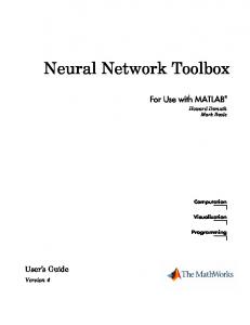
Figure 3.11: Additional memory neuron. on. Thus there is at least one Type 3 neuron which in the initial state was off. If none of these neurons turn on, then for every such neuron, z, κez = Kij − 1, κrc z = 1, sz = −1, and Iztot > 0.25, contradicting that none are on. So, at least one Type 3 neuron will turn on. Suppose more than one of these neurons turns on, then since all of the Kij −1 Type 1 neurons will remain on, κez ≥ Kij for all neurons, and Iztot < 0.25. This implies all neurons are off, a contradiction. Thus only one neuron turns on, if not a Type 2 then certainly a Type 3. If the neuron that turned on is Type 3, then it is blocked by some neuron z in the same row or column. Since neuron z was on before, it is now a Type 3 neuron. Since sz = 1, by (3.4) it will turn off. Thus, the proof of the theorem is complete. We digress at this point to discuss an interesting modification of the neural network defined so far. One function that needs to be performed after every calculation is the inverting of si for all neurons corresponding to calls that were rearranged. One way to do this automatically is to add to each neuron i in the network a memory neuron. Figure 3.11 shows the modified circuit. The connections between a neuron and memory neuron pair are chosen so that if the neuron is on, then the memory neuron is off, and if the neuron is off, then the memory neuron is on. The memory neuron gets its name since (C/λ)memory � (C/λ), resulting in a much longer time constant. Because of this, the memory neuron remains in its state for a long time
51 after the primary neuron changes. By making the connection to neuron i from the memory +0.5, it serves exactly as si . This shows how we can use non-uniform time constants and exploit them to our advantage. We assume that all of these networks incorporate si in this way. The example of a rearrangement from Figure 3.9 is redone using a neural network in Figure 3.12. This shows all the basic features of the circuit. The evolution of the neural circuit is virtually identical to the algorithm described by Paull. Theorem 3.2 shows that the neural network, as it is defined, follows Paull’s algorithm exactly, except that it does not alternately rearrange the same two symbols Q and R defined in step one of the algorithm. The previous example works, though, since there are only two symbols to arrange (i.e., n = 2). In general, for n > 2, this exception results in states that violate the constraints. Furthermore, it can result in rearrangements involving many more than 2r rearranged calls. The network needs to globally communicate the symbols Q and R to alternately rearrange. We are assuming that no Type 2 neurons exist at (i, j), otherwise by Theorem 3.2 we know that the neural network will behave correctly. Figure 3.13 shows the modifications necessary to force the network into following the algorithm. The additional circuitry consists of a set of detectors labeled D1, D2, and D3. Figure 3.13a shows the D1 detector added to each neuron-memory neuron pair. The connections to a D1 are such that it only turns on if both neurons in the pair are on. This occurs only if the neuron was off and recently turned on, thus the D1 detectors detect neurons that turn on during the course of the rearrangement. Figure 3.13b shows the detectors located at the end of each row of the neuron grid. A similar set appears at the end of each column. For each symbol, Q, there are detectors denoted by D2Q , and D3Q . The D2Q detectors simply collect the outputs of all of the D1’s associated with symbol Q in this row. It turns on if any of these neurons turn on. The output of D2Q is a small positive signal fed back to each of the neurons labeled Q in every other row. Thus a neuron i turning on causes its D1 neuron to turn on, which in turn causes the associated D2Qi neuron in row r˜i to turn on, which then feeds a small positive signal back to the neurons labeled Qi in every
52
Figure 3.12: Neural network solving blocking situation.
53
Figure 3.13: Additional circuitry to force the network to follow Paull’s algorithm.
54 other row. This means that once a symbol is placed, it will be favored over otherwise equal symbols in all subsequent rearrangement steps. As a result, the first symbol placed chooses the first symbol with which to rearrange. We need to choose an appropriate second symbol to rearrange with. For a blocked call request at entry (i, j) (i.e., no Type 2 neurons), a sufficient condition for choosing symbols Q and R to rearrange is that they can not appear together in row i nor in column j. The neuron that turns on will force another neuron either in the same row or the same column to turn off. Assume that it is in the same row. Since there are no Type 2 neurons, any symbol not appearing in row i will be in column j. This implies that if the symbol placed in this second rearrangement is not in row i then it must be in column j, and will satisfy the conditions for the second symbol chosen to rearrange. The D3Q neurons guarantee this result, as we now show. A D3Q neuron turns on if a neuron Q is on in the same row and one of the other D2R , R 6= Q, are on, that is, if symbol R was placed in this row and symbol Q is also in this row. The output of D3Q is a small negative signal to each of the neurons labeled Q in this row. Thus, in the second rearrangement step, neurons corresponding to symbols already placed in this row are disfavored. Further, out of the remaining neurons, the neuron that turns on will, through its D1 and D2 detectors, favor neurons with the same symbol in all further competitions. Thus the network chooses two appropriate symbols to rearrange in the first two rearrangement steps, and subsequent steps will favor these two symbols. Since the detector signals add to all of the neurons in the same row, an efficient way to distribute this signal is to add them once to the inhibition summers at the end of the row as shown in Figure 3.13. Each neuron receives control signals from up to 2(r − 1) D2 and two D3 detectors. To guarantee our previous results, we require that the total control signal, xi , from the D2 and D3 detectors never exceeds the limit given by |xi | < 0.25. Figure 3.14 shows an example of this network in action. Again the neural network follows the algorithm as stated by Paull. We check that the solution is reasonable. Table 3.1 tallies the number of neurons
55
Figure 3.14: Solving the rearrangement problem for n = 3.
56
Table 3.1: Tally of the neural rearranger size. Total Number of Type Total Number Connections from Neuron r2 n 6r2 n Memory r2 n 2r2 n D1 r2 n 2r2 n 2 D2 2rn 2r n + 2rn2 − 4rn D3 2rn 2rn 2 2 Total 3r n + 4rn 11r n + 2rn2 − 2rn
and connections as a function of the parameters n and r. Under the assumption √ that r ≈ n ≈ N , the number of neurons and the number of connections are both O(N 3/2 ). This is equivalent to the number of crosspoints in the switch. The time to √ find the rearrangement is given by Paull’s algorithm and is O(r) = O( N ). Therefore the neural network solution to the switch rearrangement problem is approximately as complex as the switch itself, but no more complex, and uses time as fast as the best algorithm. As a conclusion to this section, we describe an interesting application of this controller. To reduce the number of crosspoints below the minimum possible in a three stage Slepian switch, we can construct each of the center stage switches out of a smaller three stage network. This recursive construction, if taken to its limit, leads to a switch constructed solely out of 2 × 2 crossbars: N/2 2 × 2 inlet/outlet stages connected to two center stage switches that each have N/4 2 × 2 inlet/outlet switches, and so on. This is known as a Beneˇs network [1]. It has a total of O(N log(N )) crosspoints. How can we find routes through this switch? We construct a hierarchical neural network. The first level is the neural network of Figure 3.10. The outputs of this network are the on neurons that indicate the necessary connections through center-stage switches A or B. But, these requests can be used to control the next level, the two smaller controllers for switches A and B. Each of these in turn control their own two center stage switches. Continuing in this manner until all the center most 2 × 2 switches are reached. Thus we can use the
57 neural network to control the many switches that conprise this efficient but difficult to control switch design.
3.7
Conclusion
This chapter took the design techniques from Chapter 2 and implemented two switching control algorithms using neural networks. In both cases we were able to take a circuit with known characteristics, the Winner-Take-All, and utilize its capabilities within a larger neural system. It was a primary means for communicating the many constraints of the problems between the neurons in our solutions. In large multistage switches, determining the existence of a route through a switch and, if possible, determining the route itself is a time consuming problem with conventional computer architectures. We defined the simplest brute force search technique and designed a massively parallel neural algorithm that was able to implement this technique. In a three-stage rearrangeable switch, previously placed calls may have to be rerouted before a new call can be put up through the switch. Using a known optimal algorithm, we designed a neural network solution that has complexity (in terms of the number of nodes and connections) on the same order as the complexity of the switch (in terms of the number of crosspoints). By assuming nonuniform time constants in the neurons, we showed that the consequent time delays could be used to computational advantage. We discussed a recursive extension to the three-stage rearrangeable switch that utilizes the ability of neurons in one network to program the neurons in another network. In both solutions, one freedom is that the various “programming” neurons (e.g., the feedforward neurons in the first problem, and the detectors in the second) could easily be implemented with components other than neural networks. For instance, the feedforward neurons could be optical components that are ideal for the interconnect between stages. The detectors could be standard digital logic. In any case, as long as the signals that they introduce are within the limits defined in the neural solutions,
58 the system will still function correctly. The neural components can be concentrated where they can excel: as highly interconnected feedback elements. The solutions described here show that neural networks can be applied to practical problems. We emphasize that although each instance of these problems requires a different neural network, the solution is well defined, even for large-size problems where the parallelism of the neural network is most advantageous.
59
Bibliography [1] Beneˇs, V. E., Mathematical Theory of Connecting Networks and Telephone Traffic. Academic Press, New York, 1965. [2] Inose, H., An Introduction to Digital Integrated Communications Systems, Univ. Tokyo Press, 1979. [3] Schwartz, M., Telecommunication Networks: Protocols, Modeling, and Analysis, Addison–Wesley Pub. Co., Reading, MA., 1987. [4] Beneˇs, V. E., On Rearrangeable Three-Stage Connecting Networks, Bell System Technical Journal, Vol. 41, 1962, pp. 1481–1492. [5] Paull, M. C., Reswitching of Connection Networks, Bell System Technical Journal, Vol. 41, 1962, pp. 833–855.
60
Chapter 4 Banyan Network Controller The distant goal of “neural networkers” is to understand how to store, retrieve, and process data in neural networks; ultimately to characterize the types of data that need to be stored, to know best how to represent them, and to see how to design such machines that accomplish it with the greatest engineering ease. —J. S. Judd [1]
4.1
Introduction
This chapter will develop a neural network design, starting from the original problem analysis and formulation, proceeding through the design stage, continuing on to implementation considerations and further applications of the networks developed. Along the way we will develop many interesting results related to switching and queueing theory, and will finish with a feasible design of a 1024 × 1024 packet switch controller based on neural network principles.
4.2
ATM switching networks
This section gives a general background to the ATM (Asynchronous Transfer Mode) switching environment, and introduces the fundamental problem of blocking and queueing. It also motivates why we need a new approach. A Broadband Integrated Services Digital Network (B-ISDN) consists of two major parts: optical transmission with a Synchronous Optical Network (SONET) [2], and switching with an ATM [3] switch. Although current transmission rates are already
61 several gigabits per second, the ATM switching fabric at present can function at rates up to only a few hundred megabits per second. The broadband network research community has therefore spent much time and effort on the design of ATM switch fabrics. One approach in designing ATM switch fabrics is to use interconnection networks [4] that were originally designed for multiprocessor parallel and distributed processing. There are several different interconnection networks; e.g., Banyan, Baseline, Buffered Memory, Delta, and Shuffle Exchange [4, 5]. Among them, the Banyan network is the most popular to be used as a basic building block in ATM switch fabric designs, although Buffered Memory switches are gaining in popularity due to their simplicity in concept. In an ATM network, unlike the circuit switching of Chapter 3, bursty and continuous data are segmented into small fixed-length units called ATM cells. These cells will be our basic unit that the ATM switching network processes. The data rates are approximately 150Mbs and the cell sizes 53 bytes (424 bits) [3]. This implies that any cell processing must be completed in less than 2.8µsec. We assume there exist some external interface modules that assign each cell entering the switching network an output destination address. Within every ATM network, blocking must occur due to what is called output blocking. If two or more inputs to the network have cells with the same destination address, their cells will be routed to the same output at the same time and hence collide. This is output blocking. Output blocking cannot be avoided, so blocked cells must be buffered somewhere. The location of the buffers affects the queueing characteristics of the network. Although not optimal, we will assume that cells are buffered at each input since this produces the least complicated network. This will be discussed further in the section on queueing. A controller is needed to choose which cells to send at an instant and guarantee that all the destination addresses are distinct at that instant. The choice of controll algorithm is important. The simplest controller uses first in first out (FIFO) queues, and chooses a non-blocking set of cells from the head of the queue. Unfortunately,
62 this scheme suffers from a statistical impediment called “head-of-line” blocking [6] that ultimately results in each input transmitting significantly less than one cell per time slot. To achieve higher rates, more sophisticated controllers use bypassing. In this scheme, cells with different destination addresses further back in the queues are transmitted instead, if doing this avoids blocking. While this increases the maximum throughput rate over that of the FIFO scheme, many of the proposed bypass control schemes still have the problem that the maximum throughput per input is significantly less than one cell per time slot [7]. The controller is further complicated when the switch can not transmit every possible permutation of the inputs, that is, there are sets of cells with distinct inputs and outputs that can collide due to overlapping paths through the switch. This is internal blocking. ATM switches that have no internal blocking (but still the unavoidable output blocking) we denote as non-blocking, otherwise they are blocking. We note that implicitly most switching networks have a third form of blocking, input blocking: only one cell may enter each input per time slot. Some control schemes treat the internal and output blocking separately. For example, to avoid internal blocking within the Banyan network, a so-called Batcher sorter network is used to preprocess the incoming cells of the ATM switch fabric [8, 7]. In this scheme, the cells are first sorted in such a way so that they arrive to the Banyan in an order that avoids internal blocking. But this sorting scheme suffers from several deficiencies. Foremost among these is that it is even more complex than the Banyan network itself. This is true not only in terms of the number of switching elements, but also, since these elements must make comparisons between the destination addresses to perform their sort, a precise cell bit alignment must be maintained through the sorting network. Furthermore, some output blocking still occurs anyway, and queueing and a controller are still required. As an alternative to the Batcher network, we combine the processing for both internal and output blocking into a single controller. This controller utilizes the state of all the input queues in a bypass scheme that increase the throughput of the ATM switch as a whole. We define a useful class of switching networks to which this method
63 applies. We also design a neural network implementation of the controller. By using the massive parallelism of the neural network, we can complete each computation quickly. Before we develop these ideas we digress to discuss a particular ATM switch architecture.
4.3
Banyan Networks
We base this section on the work of K. H. Liu [9, 10]. It is included for completeness, and to set up notation for future sections. The Banyan network considered consists of n = log2 N stages composed of 2×2 non-blocking switching elements (see Figure 4.1). The topology of the Banyan network can be generated in a recursive way. An N × N Banyan network can be viewed as a first stage with N/2 switching elements, followed by two (N/2) × (N/2) Banyan sub-networks. The connection between the first stage and the following blocks is the “Banyan Exchange.” This will be defined later. The Banyan network has the routing property. Rather than a global router, the individual switching elements themselves are able to route cells correctly much as in the old step-by-step telephone switches. The routing strategy for a switching element in stage k is to look at the kth most significant bit in the destination address of a cell and send the cell to the “top” outlet if the bit is 0, and to the “bottom” outlet if the bit is 1. Figure 4.1 shows an 8 × 8 Banyan network, and an example of the self routing. A cell arrives at input 010 and is destined for 101. In the first-stage switch it is routed to the bottom outlet since the first bit of the destination address is 1. In the second stage it is routed to the top outlet since the second bit is 0, and in the last stage it is routed to the bottom outlet since the last bit of the destination address is 1. Note how the successive address bits automatically direct the cell to the correct output destination, and how the cell would arrive at outlet 101 no matter what inlet it started at. The topology of the Banyan network can be abstracted and described in terms of functions on the input and output addresses of the cells. We assign a label, (I, D), to each cell at the input of the network, where I = in in−1 . . . i1 is the cell’s input address
64
Figure 4.1: An 8 × 8 Banyan switching network showing self routing of cell (010,101). and D = dn dn−1 . . . d1 is the cell’s output (destination) address; both are written in n-bit binary (n = log2 N ). As shown in Figure 4.1, we number the inlets and outlets to each stage 0 to N − 1 sequentially in n-bit binary. Define L as the locator label n-tuple of a cell as it is transmitted through the network. L indicates the address of the input or output to the switching stage at which the cell is currently located. The Banyan network can be represented as bitwise operations—one corresponding to each of the stages of switching elements and to each of the sets of links between stages—that transform L from L = I at the input to L = D at the output. This is effected by defining a set of topology defining rules [5]. The operation Rk of switching stage k is a binary operation, a function of a cell’s address at the input to the stage and its destination address D: Rk (an an−1 . . . a2 a1 ) \ (dn dn−1 . . . d2 d1 ) = (an an−1 . . . a2 dn−k+1 ). This “replacement operator” defines the self-routing of the cells. In Figure 4.1 we see how the cell at input 2 (010) of Stage 1 is sent to output 3 (011), since the MSB
65 of D is 1. The Banyan Exchange connection between the kth and (k + 1)th stage switching elements is: Bk (an an−1 . . . a2 a1 ) = (an an−1 . . . an−k+2 a1 an−k an−k−1 . . . a2 an−k+1 ). This operator simply swaps the least and the kth most significant bits. (We use the usual convention that ax ax−1 . . . ay is null when x < y.) Continuing with our example, the Banyan exchange routes the output of the first stage at output 3 (011) to the input of the first stage at 6 (110). By concatenating these operators together, the Banyan network is represented as: Rn Bn−1 Rn−1 . . . B2 R2 B1 R1 (I) \ D. Using these operations, we see that the locator label L for our example cell is transformed through the sequence (010), (011), (110), (110), (101), thus ending at the desired destination (101). In general, for an n stage Banyan network, we define: 4
Lk (I, D) = dn dn−1 . . . dn−k+2 in−k in−k−1 . . . i2 dn−k+1 .
(4.1)
This is the locator label at the outlet of stage k of a cell from inlet I to outlet D. For consistency, we define the input as Stage 0, with L0 (I, D) = I.
4.4
Blocking Constraints and Deterministic Switches
In this section, we define a general class of Banyan-like switches that we denote as deterministic. For a given switch architecture, let S = {(I, D)} be a set of cells such that every cell in this set is mutually blocking, that is, given any two cells in S, these cells collide somewhere in the switch. Such a set we call a constraint set. For deterministic switches, these constraints are simple to define, and can be used to completely define blocking. We will later investigate the blocking for two switch architectures from within this class. A switch is deterministic if:
66 A. The switch is composed of non-blocking square switch nodes. B. The nodes can be arbitrarily interconnected, but any switch input or output has only a single link to one of these nodes. C. Between each input and output there is exactly one route (defined in terms of links and nodes). A Banyan network is a deterministic switch composed of stages of 2 × 2 nodes. A non-blocking switch is a deterministic switch with a single node—the switch—that has links to the inputs and outputs. Omega networks, baseline networks, and flip networks are all topologically equivalent to the Banyan network and therefore also deterministic switches [5]. To define the constraint sets, we note that whenever two cells both attempt to use the same link between two switches, there is a collision, and thus blocking. These two cells will always collide, since they have only one choice for routes, and both routes are through this link. Each of the switching elements are non-blocking, as long as only one cell arrives per input and leaves per output. Therefore, none of the cells are blocked if and only if there is no link used by more than one cell. Let LA = {lj }, be the set of links in a switch with architecture A. Each link, lj , in the switch defines a constraint set, Sj = {(I, D)| the route from inlet I to outlet D uses link lj }. Using these constraint sets, our definition of non-blocking is clear: Definition: A set of cells, C = {(I, D)}, is non-blocking if and only if each set, Sj , contains at most one (I, D) ∈ C. For the Banyan switch, LBanyan = {ljk }, 0 ≤ k ≤ n, 1 ≤ j ≤ N , where ljk is the link connected to the jth outlet of the kth stage of switches. In the case of the nonblocking switch, the only links are the input and the output links. In terms of the Banyan definition of ljk , LNB = {ljk }, where k ∈ {0, n}, and 0 ≤ j ≤ N .
67 From this labeling, we can define the constraint sets using (4.1): Skj = {(I, D)|Lk (I, D) = j}. 4
These sets have an interesting interpretation. For each k, there are N different Sjk , since there are N different links between each stage. At any stage, each cell uses only one link, so Sjk ∩ Sik = ∅ for all i 6= j. Since at any stage a cell must use some link, SN −1 j=0
Sjk is the set of all possible input-output pairs. Thus we have shown that each
Lk , 0 ≤ k ≤ n, partitions the N 2 input-output pairs into N equivalence classes. A more graphical interpretation can be gleaned from the following construction. Given a set of cells C = {(I, D)}, we create a binary N × N cell matrix by placing a 1 at entry (I, D), ∀(I, D) ∈ C. Using this matrix, Figure 4.2 shows the n + 1 = 4 different sets of equivalence classes for N = 8. Let C A = {C : |C| = N and C is non-blocking in switch architecture A}. This is equivalent to the set of permutations realizable by the switch. From [9, 10], we find the number of these non-blocking sets for the Banyan (here as before N = 2n ):
|C Banyan | = 2
nN 2
= N N/2 .
(4.2)
To compare the Banyan network to a non-blocking network, we note that the Banyan network has n + 1 levels of blocking, one for each set of links between stages. The non-blocking network has only two levels of blocking; input and output. Since the non-blocking network can transmit any permutation, C NB = N !. To get an idea of the size of C Banyan relative to the set of all permutation matrices, we use Sterling’s √ √ formula to show C NB = N ! ≈ 2π2nN −1.44N +n/2 = 2πN /21.44N (C Banyan )2 . Before investigating the implications of these differences further, we discuss some background on queueing architectures for switching networks.
4.5
Queueing
This section will introduce the queueing model for our system. We will investigate other queue control methods that have been proposed for this system, and then
68
Figure 4.2: The equivalence classes induced on the 8 × 8 input matrix by each stage of links in Figure 1. The numbers in the matrix indicate which link a cell uses at stage k.
69
Figure 4.3: The queueing model.
introduce our method, applicable to the class of deterministic switches. We show that the method has a throughput per inlet arbitrarily close to one cell per time slot. As discussed in the introduction to this chapter, even if a preprocessor removes all internal blocking (if any exists) leaving only output blocking, cells must be queued to prevent losses. We assume a model as shown in Figure 4.3. The cells arrive at an input according to some random process, and each cell is destined for one of the outputs according to a second process. Cells that are blocked and can not be sent are queued at each input. We assume that the inputs have independent and identical arrival processes. For the purposes of this chapter we consider two arrival processes. The simplest is a Bernoulli process, where one cell arrives at the beginning of each time slot with probability α. The second arrival process that we consider is a batch process where cells arrive in batches, every cell within a batch destined for the same output [11]. The number of cells within each batch is geometrically distributed, with mean batch size θ, while the number of batches that arrive each time slot is Poisson distributed, with mean number of arrivals α/θ. In either case, the destination addresses of the cells are uniformly distributed, with probability 1/N that a given output is chosen. We can view these two cases as extremes in the space of potential arrival traffic processes. For a given average number of arrivals, α, the Bernoulli case will spread the arriving traffic most evenly across the outputs and across time. The batch arrivals on the
70 other hand will tend to bring sharp concentrations of traffic both across the outputs and time. Reference [11] analyzes a single deterministic server (a 1-input switch in our terminology). That analysis showed the sharp concentrations in time. As an example, for an average burst length of θ = 10 and average arrival rate of α = 0.8 cells per time slot, to have a buffer overflow probability of less than 10−6 requires a buffer length of about 600. For the Bernoulli case, this length is only 1 (since the buffer can always send one, and at most one arrives). But as we will show, even for a 32-input Banyan with the same average number of arrivals, the necessary buffer per input is only about 30. Note that in the approach we take, the entire batch enters the queue at once, unlike other simulations [12] that assume (with reason) an additional external buffer that governs the cell arrivals so that at most one cell is transferred per time slot from the external buffer to the system. By only counting the cells in the system, the external buffer substantially mitigates the effects of the batch concentrations. For the case of a non-blocking switch, various queueing strategies are analyzed in [6] and [13]. One strategy discussed is output queueing. In this strategy, all cells are allowed to pass through the network, and multiple arrivals to an output are then queued. While this was found to be the best strategy statistically, it requires the switching network to operate at N times the transmit rate. This is undesirable in a network that is already operating at very high bit rates. Alternatively, the switching network can have multiple copies [12], but this adds undesirable complexity. For queueing at the inputs, a strict FIFO and a so called consecutive competition scheme were also analyzed in [6]. The consecutive competition strategy starts with the first cell in each queue and determines which inputs will transmit, and which inputs are blocked. Then it repeats the procedure with the second cells among the blocked queues that compete for the remaining unused outputs. This procedure can continue up to a depth w into the queue. FIFO is merely the special case of w = 1. For finite w it was found that the length of the queues became unstable even for arrival rates, α, less than one. For instance, when w = 1, the maximum throughput √ per inlet is less than (2 − 2) = 0.586 cells per time slot as N → ∞. While letting
71
Figure 4.4: The Mapping of the State of the Queues (a) to a Cell Matrix (b). A 1 is placed in (i, j) of the matrix if a cell is waiting at input queue i to be sent to output address j. w → ∞ could allow the maximum throughput to approach 1, this algorithm requires O(N w) steps to execute, and is therefore unsatisfactory for large N and w. Here we propose a new approach applicable to the deterministic switches of the last section. Given a set C of cells queueing at the inputs of the switch, we map them to an N × N cell matrix as described in the previous section, with 1’s in entry (I, D) if and only if there exists a cell (I, D) ∈ C as shown in Figure 4.4. The controller then uses the blocking constraints on the subsets Sj to choose a subset C 0 that is non-blocking. Exactly how we use these constraints to choose a C 0 is the subject of the next section. Optimally the network controller will choose a C 0 that has the maximal overlap with C. This approach has a maximum throughput of 1, even if the controller only randomly chooses a C 0 ∈ C A , and sends C 0 ∩ C. The only assumption that we make is that C A is symmetric, that is |{C 0 |(I, D) ∈ C 0 } ∩ C A | = |{C 0 |(I, D0 ) ∈ C 0 } ∩ C A | for all I, D, and D0 . By the symmetry of the switch designs, both C Banyan and C NB are both symmetric. We define the idea of the random queue manager (RQM). Given a set C of cells waiting in the queue, a RQM randomly chooses a set C 0 ∈ C A uniformly and indepen-
72 dent of C, and sends C ∩ C 0 . We also define a controller to be stable if the expected size of the queues are finite. When the queues are finite, then the throughput equals the average number of cell arrivals. With these facts in mind we show: Theorem 4.1 Given a switch with architecture A and symmetric C A , a random queue manager is stable for any average arrival rate, α, that satisfies 0 ≤ α < 1. Each input queue, I, can be decomposed into N separate queues, one for the cells waiting to be sent to each output. Focusing on the cells waiting for output D at input I, we show that this subqueue is stable under the RQM and thus so is the queue as a whole. Because the destination addresses are chosen uniformly, an (I, D) arrives every time slot with probability α/N . The RQM chooses C 0 uniformly from C A . This and the symmetry of C A implies that (I, D) ∈ C 0 with probability 1/N . Given this probability of being sent, a cell (I, D) that arrives at the head of the subqueue has an expected service time of N time slots. The utilization factor in this case is 4
ρ = (average cell arrival rate) × (average service time) = (α/N ) × N, which is stable for any 0 ≤ ρ < 1 [14, p. 19]. Since the RQM is stable for any α < 1, then any more sophisticated scheme that takes into account C is also stable with such α.
4.6
The Neural Network Solution
This section designs a neural network that chooses a set of non-blocking set of cells from the queue. The complexity of the design is calculated, and compared with another possible neural approach. For our problem, we use N 2 neurons arranged in an N ×N matrix that corresponds to the cell matrix of Figure 4.4. This is our neuron set Θ. The input to the problem is a particular cell matrix, that is, neuron (I, D) receives a +1 input if a 1 is in entry
73 (I, D) of the cell matrix, −1 otherwise. If at the end of the computation, neuron (I, D) is on, then send the cell (I, D). If more than one cell has the same (I, D), then send the first (I, D) that arrived in the queue. The neural network design follows directly from the constraint sets, Si , defined in Section 4.4. Using Θ and {Si }, we design a Multiple Overlapping Winner-Take-All according to (2.8). By definition, this has the property that no more than one neuron will be on per constraint set. Therefore, the set of neurons that are on at the end of the computation will always correspond to a non-blocking set of cells. To measure the complexity of this circuit, we count the number of interconnections. Using the construction method of Section 2.7, the number of interconnections in the P
network is O(
i
|Si |) connections. In the case of the Banyan network, there are O(N )
connections for each equivalence class, Sjk . There are (n + 1)N of these classes, so the number of connections in the network is just O(N 2 log2 N ). For the non-blocking switch, there are 2N equivalence classes. The number of classes in this case is just O(N 2 ). We can assume that the minimum circuit in either case would have at least N 2 connections, one for each neuron in the circuit. Thus, we have a circuit that is defined for any N , provably works, and is within a factor of log2 N of the smallest possible network. We contrast this with the resulting networks from the energy function approach to optimization [15]. Using that approach on the problem of choosing a non-blocking set of cells for a non-blocking switch [16], it is seen that the resulting network has O(N 3 ) connections instead of O(N 2 ), a factor of N more connections, and further, the strength of the connections must be experimentally determined for every N .
4.7
Network Prompting
The neural network gives us some flexibility in processing the cells in the network, which allows us to tailor the network to specific applications. More importantly, it allows us to modify the network to improve the choice of non-blocking sets and improve upon the statistics.
74 The definition of the network allows for inputs, Ii , other than ±1. In fact, if we set the common diagonal elements, wii = a, to zero, the network still works with positive inputs in the range 0 < Ii < 2. If two neurons, i and j, with the same capacitance, C, have approximately the same inputs from other neurons and ui (t) ≈ uj (t) at some time t, then: d(ui − uj ) = η + (Ii − Ij ), (4.3) dt where η is the sum of all the differences between the neurons. As long as |Ii −Ij | > |η|, C
we see from (4.3) that the neuron with the higher input will evolve to a higher value. For two such neurons in the same constraint set, this implies that the neuron with the greater external input will turn on. If a neuron i is in a position where other neurons are trying to turn on in each of its constraint sets, and neuron j has only one neuron (i.e., neuron i) trying to turn on out of all its constraint sets, then in this case η will not be small, but will be large and negative, favoring neuron j. This shows that the neuron with the largest input will turn on, unless doing so will block an inordinate number of other neurons from turning on. All neurons that are receiving a positive input are given a basic input I 0 . Under various conditions, a prompting signal π can be added such that 0 < I 0 + π < 2. How can we use this neural network capability? We discuss two ideas, priority and smoothing. Cells may have different priority levels. For simplicity we consider just two levels, high and low. Low priority is considered the normal case, with an input of I 0 . Neurons corresponding to cells with high priority, however, receive the prompt πH . From the previous discussion, we see that this results in a soft priority, i.e., high priority cells will be sent first as long as they don’t impair throughput significantly by preempting a large number of lower priority cells. This should prevent the deadlock behavior for low priority cells described in [6]. Further study is necessary to demonstrate this. A queue containing one cell for each destination will, depending on the architecture, always send a cell. If the queue had N cells for only one destination, the queue would be extremely limited. Snapshots of the queue state from the simulations show that in fact the latter case is the more prevalent. A simple way to decrease the average
75 queue size is to give a prompting signal πM to neurons corresponding to an (I, D) that has many cells waiting. This will smooth the number of cells waiting for each output destination in a queue, and can significantly reduce the expected queue size. These are just two possibilities of prompting; further applications include flow control, giving cells that have been waiting in the system a long time a prompt to send them along sooner, and balancing for component irregularities or degradation in the system, for example, one neuron that is slower than the others receiving a prompt to compensate.
4.8
Simulation Results
To study the behavior of the queueing system under the neural network controller, we ran a series of simulations on a MIPS M/120 computer. We outline the simulation method and present graphs of the Banyan and non-blocking switch performance. These are used as a basis for comparing with other methods of choosing a nonblocking set of cells, and with other queue control methods. Finally we compare the Banyan and the non-blocking switches to each other to show that with a powerful controller such as the neural network, these switches have similar performance, i.e., the Banyan is almost as good as the non-blocking switches. For a given switch architecture and size, N , the simulation set up N input queues, N 2 neurons, and defined all the constraint sets and resulting weights; wii = 0 was used. The simulation consisted of a sequence of time slots. Each time slot comprised the following steps: 1. Generate a set of arrivals for each input queue according to the chosen arrival process. Add the arrivals to the queues. 2. Create a cell matrix based on the current state of the queues. 3. Using the cell matrix, set up the inputs to all of the neurons. 4. Let the neural network settle on a solution.
76 5. Determine the neurons which are on, and remove the corresponding cells from the queue.
Statistics were recorded on the states of the queues after Step 1, as well as the time in the system of cells sent in the last step. Consistency checks were also made to guarantee that the the constraints were always met (after debugging, they always were). The simulation of the neurons deserves further discussion. Step 4 consisted of numerically integrating the differential equation in Equation (2.1). Several methods were tried for this; Euler’s method, fourth order Runge-Kutta method with adaptive step size [17, Sec. 15.2]; and Richardson extrapolation with the Burlirsch-Stoer method [17, Sec. 15.4]. Euler’s method suffered from always taking too big or too small steps. The Burlirsch-Stoer method suffered from trying to extrapolate too much information from the highly non-linear neuron functions. The Runge-Kutta method was the most satisfactory. At the start of the simulation, the capacitances were assigned the value ex , where x was chosen uniformly from (−0.05, 0.05). At the start of Step 4 of each time slot, the neuron states were initially set to a small number near zero chosen uniformly from (− 0.05 , 0.05 ). The exact values here were not imporλ λ tant; they were chosen only to add a small amount of noise to the system to prevent instabilities in the simulation. Since the inputs, Ii , were chosen to be ±1, by (2.11), a neuron which turns on (κi = 0) will have a net input of 1. This implies that the internal state approaches
1 . λi
For the purposes of timing, the network was considered to have settled when, after an initial period, all of the neuron states were more than
1 2λi
away from zero. For
each simulation run, we recorded the maximum, minimum, and average settle times. In calculating the derivative, we took advantage of the implementation techniques of Section 2.7. By summing the outputs of all of the neurons in each constraint set once and then for each neuron adding the resulting sums from the constraint sets to which it belongs, the complexity was reduced by a factor of |Sjk | = N . The sigmoid function used was the hyperbolic tangent function. The gain was always chosen so
77
Figure 4.5: Demonstration of smoothing for simulations of Bernoulli traffic into an 8-input Banyan network with various controllers. that it was larger than the value in Table 2.1 with � = 0.5. In the previous section, we discussed the benefits of smoothing the input. Figure 4.5 shows such a comparison for an 8 × 8 Banyan network, using I 0 = 1 and πM = 0.3 when two or more cells of the same (I, D) are waiting. The 8 × 8 size was chosen so that we could compare it to an optimal controller, i.e. one that exhaustively searches all of C Banyan and sends the largest non-blocking set. Figure 4.5 shows that the prompting brings the neural network closer to the optimal controller in performance. Because of this benefit, we will assume that all neural controllers use this smoothing. The choice of πM = 0.3 followed from testing of various values between 0.0 and 0.5 in increments of 0.1. Within this range 0.3 was the best, slightly better than 0.2 and 0.4 which were significantly better than values larger and smaller. Using the computer simulator, we tested the neural network on Banyan and non-
78 blocking networks with 2, 4, 8, 16, and 32 inputs. A simulation consisted of 10,000 time steps of cell arrivals at a chosen arrival rate α. The average input queue sizes under Bernoulli arrivals are plotted as a function of α in Figure 4.6. These results show that high throughput rates can be maintained with only modest queue sizes, even for large switching networks. Figure 4.7 show the same graphs, but now with batch arrivals (the extra plots on the figure will be discussed later in this section). The average batch size was θ = 10. As expected, because of the more sporadic arrivals, the average queue sizes are much larger. The simulations were not as extensive in this case for two reasons. The first is that even though we simulated for over 10,000 time steps, the data contained a large variance, and was not as informative. This was seen by observing subsamples of the data. Increasing to 100,000 time steps only decreased the variance marginally. The second reason was that except for at the larger α, the plots were very close, often crossing each other several times. Since this is a work-conserving system the average wait time, W (not graphed), of a cell can be calculated in terms of the average queue length, L, using Little’s formula: W = L/α [14, p. 17]. We compare the neural networks method with two other methods of choosing a non-blocking set of cells to send. The simplest method to compare with is a greedy algorithm. In this algorithm, we randomly choose one cell to send from each queue, throwing out any blocked cells one by one, until the remaining set of cells is nonblocking. The queueing behavior for this method we consider an upper bound. As a lower bound, we might consider a simple exhaustive search of all C 0 ∈ C A to find the set with the largest |C 0 ∩ C|, but this becomes computationally prohibitive for switches with more than 16 inputs, where even for the Banyan the possible number of non-blocking sets is 2
Nn 2
≈ 4.3 × 10⁹ . In the case of the non-blocking switch,
the problem of finding a maximal non-blocking set of cells to send reduces to the cardinality graph matching problem. This latter problem has a known polynomial time algorithm that solves it exactly [18]. Given a bipartite graph [19], a set M of edges is a matching if no two edges in M are incident to the same node. The cardinality matching problem is to find
79
Figure 4.6: Average queue size vs. average number arrivals for simulations of Bernoulli traffic into Banyan (a) and non-blocking (b) switches with 2 to 32 inputs.
80
Figure 4.7: Average queue size vs. average number arrivals for simulations of batch arrivals into various networks. the matching with the largest number of edges. The reduction of the maximal nonblocking set problem to cardinality matching is simple and direct. Given an N × N cell matrix, C, construct a bipartite graph B = (X, Y, E), where X = {x1 , x2 , . . . , xN } and Y = {y1 , y2 , . . . , yN } are two sets of vertices, and E = {(xi , yj )} is the set of edges. If (I, D) is 1 in the cell matrix, then (xI , yD ) ∈ E, and vice versa. If (xI , yD ) ∈ M then we send cell (I, D). For a matching M ⊂ E on B, (xI , yD ) ∈ M implies this is the only edge in the matching incident on node xI and on node yD . The constraints placed on a non-blocking set of cells for a non-blocking switch require no more than one cell per input and one cell per output. So the edges in a matching M correspond to the cells in a non-blocking subset of C. Figure 4.8 shows graphs of the average queue size for the greedy, neural network, and optimal method on a 32-input non-blocking switches. The results show, we think
81
Figure 4.8: Performance range for simulations of Bernoulli traffic into a 32-input non-blocking switch. as expected, that the neural network produces results intermediate between the two extremes. The range of values is not great, suggesting that we might consider the simple greedy algorithm. But even this has O(N 2 ) time complexity. Assuming that the algorithm requires just N 2 machine cycles to find a non-blocking set on some serial machine, in order to complete this operation in less than the 2.8µsec between cell transmission times would require a clock speed of over 350MHz for a 32-input switch. This rules out this algorithm, and the even longer matching algorithm (time complexity O(N 5/2 )), for all but the smallest switches. We now compare the neural network with alternative controlling schemes using a 32-input non-blocking switch. The first scheme is the sequential competition scheme described in Section 4.5 (w = ∞), while the second is an output queueing scheme where all cells are allowed to pass through the switch to the outputs [6, Equation
82
Figure 4.9: A comparison of different control architectures on 32-input switches with Bernoulli arrivals. (21)]. These are all plotted on the same graph in Figure 4.9 (along with a plot for the neural network on the Banyan switch). Of the three, the sequential competition scheme, even with this optimal window size, is the worst. The output queueing is the best, as little as half the queue of the neural controller, but at the expense of a more complicated switch. From our discussion in the introduction, the cost of gaining this at best factor of two gain in performance is an N times more complicated switch. For large N this can be an expensive trade-off. An interesting implication follows when we directly compare the performance of the Banyan network to that of a non-blocking network such as the Batcher Banyan combination. As discussed already, both will have queueing due to output blocking, but the Banyan network has additional internal blocking. For the Banyan we use the neural network with prompting as just described. For the Batcher Banyan we
83 use the sequential competition scheme and a neural network controller. We compare them using switches with 32 inputs. Results for these three are shown in Figure 4.9. This graph shows that the non-blocking network out-performs the Banyan network by a factor of two to three. This was for the case of Bernoulli arrivals. In the case of Batch arrivals, Figure 4.7 plots both the Banyan with neural network controller and the non-blocking switch with optimal matching controller. In this case we see that again the difference in performance is a factor of two to three. From an engineering standpoint, a more relevant parameter than the average queue size is the length of the buffer, B, such that the probability of losing a cell due to a saturated buffer is less than a given level, PL . Appendix 4.A derives a method for estimating an upper bound on B as a function of PL using data on the distribution of the queue size recorded during the simulations. Using this method, we construct Table 4.1 of upper bounds on B. With this table as a measure, we see that the Banyan network is still within a factor of two to three of the non-blocking switch. Note, however, that the necessary buffer size in the case of batch arrivals is significantly larger, by a factor of 100 or more. Although the non-blocking switches outperform the Banyan network, this better performance should be viewed in light of the extra complexity of a non-blocking switch. In many cases it would be simpler to use the longer queues with a Banyan network than to add the additional hardware necessary to make the network nonblocking.
4.9
Implementation Considerations
We show that each input queue can interact with the neural network in an independent and efficient manner. We also show that the constraint sets in the case of the Banyan network possess a regularity that can simplify the construction of the controller. Figure 4.10 shows a schematic of the architecture for a single input queue. It consists of the queue itself; the controller logic; the neural network; and a small amount of memory to hold a pointer to the first instance and the number of each type of cell.
84
Table 4.1: The Length of Buffer B Sufficient to Reduce Cell Loss Below PL for Various Combinations of Offered Traffic, α, and Switch-Controller Pairs. (a) Bernoulli traffic. Switch Type: Controller: PL 8 Input 10−3 Switch 10−6 10−9 32 Input 10−3 Switch 10−6 10−9
Banyan Non-Blocking Neural Net Matching Neural Net α = 0.50 0.75 0.90 0.50 0.75 0.90 0.50 0.75 0.90 5 11 30 4 7 16 4 8 21 8 20 57 6 12 26 7 14 32 12 29 84 9 17 37 10 19 44 7 18 41 3 6 15 4 9 32 12 28 56 6 11 26 7 17 53 17 37 70 8 15 36 9 22 74 (b) Batch arrival traffic.
Switch Type: Controller: PL 8 Input 10−3 Switch 10−6 10−9 32 Input 10−3 Switch 10−6 10−9
Banyan Neural Net α = 0.50 0.75 210 280 490 470 770 670 160 560 300 1100 440 1700
0.90 1200 1500 1700 870 1200 1600
Non-Blocking Matching 0.50 0.75 0.90 140 230 740 280 390 1700 440 540 2600 130 260 680 270 510 1300 400 750 1900
85
Figure 4.10: A schematic of the queue architecture for one of the input queues. Since the memory keeps track of the first instance of each type of cell, all cells sent to the same destination remain in arrival sequence. The following table lists the processing algorithm at time step τ . Initialization Queue Control reads the destination, DN ew , of newly arriving cell. If #DN ew = 0 then: Set Pointer for DN ew Toggle Latch DN ew to +. Increment #DN ew Concurrent Release neural network. If Dτ −1 was sent last time, Processing Read destination address Dτ . update pointer to next Dτ −1 . Post Send cell at pointer for Dτ . Processing Decrement #Dτ . If #Dτ = 0, change latch Dτ to −. In every time slot, at most one cell can leave, and cells for one destination can arrive. Since the latches retain their state from one time slot to the next, at most two latches are modified in any time step. For maximum throughput, the three steps in
86 this table must be completed in less than one time slot, 2.8 microseconds. We assume that the capacitance, C, is proportional to the number of connections per node, and the base capacitance is 2pF. The resistance of a connection we assume is 100KΩ. This results in a worst case settle time over all simulations of 250 nsec. This allows sufficient time for the other processing requirements. The limiting step in this process is the updating of the memory about Dτ −1 . This requires a search of the queue to find the next cell destined for Dτ −1 , which scales with the size of the queue but not with the number of inputs, N . This search-time limit can be removed if necessary by using a larger pointer memory that stores the location of each successive cell for each destination. As a final point, we describe an efficient layout of the neurons for the Banyan controller. The equivalence classes in Figure 4.2 all occur in contiguous blocks of neurons. Note, though, that the numbering of the rows (inlets) is not in sequence. We claim that we can always reorder the rows or columns so that the equivalence classes are in blocks. Formalizing this notion of blocks, for an N × N matrix of neurons, (νrc ), a set S of neurons is said to be a block if there exist integers r ≤ r0 and c ≤ c0 such that νlm ∈ S if and only if r ≤ l ≤ r0 , and c ≤ m ≤ c0 . Theorem 4.2 For an N = 2n -input Banyan network, we can always find a single permutation of the labels on the rows and columns so that all of the constraint sets Sjk are blocks. Proof: Recall Section 4.3. For a particular Banyan network configuration, the switches in stage k replace ixk by dyk . For a column labeled D = dn dn−1 . . . d1 , rearrange the order of the bits and label the column instead dy1 dy2 . . . dyn . Similarly, relabel the rows from I = in in−1 . . . i1 to ixn ixn−1 . . . ix1 . We show that this is the desired permutation of the rows and columns. After stage k, the locator label, L, of a cell is composed of the bits ixn ixn−1 . . . ixk+1 from the input address and the bits dy1 dy2 . . . dyk from the destination address. For simplicity we will assume that L = ixn ixn−1 . . . ixk+1 dy1 dy2 . . . dyk . In this case, Sjk = {(I, D)|L = ixn ixn−1 . . . ixk+1 dy1 dy2 . . . dyk = j}.
87 This set includes all neurons, νID , such that ixn ixn−1 . . . ixk+1 00 . . . 0 ≤ I ≤ ixn ixn−1 . . . ixk+1 11 . . . 1, dy1 dy2 . . . dyk 00 . . . 0 ≤ D ≤ dy1 dy2 . . . dyk 11 . . . 1. But, for the permutations we defined, these correspond to contiguous rows and columns and by definition this is a block. The proof is general enough to include all switching networks that are topologically equivalent to the Banyan, such as the baseline network. In our case yk = n − k + 1, implying that the columns are unpermuted. For the rows, x1 = 1 with xk = n − k + 2 for k > 1. For N = 8, this implies that the most significant two bits are simply permuted. The fact that the constraint sets for the Banyan network controller are blocks can greatly simplify the layout.
4.10
Buffered Memory Switches and Large Switch Designs
In this section, we discuss buffered memory switches and show how we can use them to design a large ATM switch. A buffered memory switch is simply a high speed memory device that reads in all the arriving cells and reads out previously stored cells to the appropriate output lines. The memory can operate at ATM rates (≈ 150 Mbs) by first converting the cells from serial to parallel and then sending the cells one by one into the memory, gaining a data slow-down factor of cell size 424 = , number of input lines n where 424 is the number of bits in a cell. So far the largest buffered memory switch proposed is n = 32 [20]. This results in a manageable internal data rate of 12Mbs. The first advantage of these switches is that in effect they are utilizing output queueing with the improvement in queueing statistics shown in Figure 4.9. The second advantage is that, due to the trunking effect of the shared memory, they have a significant reduction in the buffer size per port for a given accepted level of cell loss. For n = 32, this is a reduction by a factor of 7 as shown in [20]. For larger
88
Figure 4.11: The buffered-memory Banyan hybrid switch. n, this reduction factor is even larger. Unfortunately, due to the current state of technology, the possibility of going to larger n is restricted by memory speeds. One way to increase the size of the switch is to build larger switches from stages of the buffered memory switches as described in Chapter 2. The problem is that the buffered memory switch is an expensive component. We propose a hybrid buffered-memory Banyan switch that would have the advantage of reduced buffer requirements and reduced blocking over the original Banyan, and allow for larger switch sizes than can easily be achieved by a single buffered memory switch. Figure 4.11 shows the architecture. It consists of two stages of switches, a first stage of buffered memory switches and a second stage of Banyan switches. We show that this hybrid switch can be controlled. The buffered memory switch acts simultaneously as a queue and an initial switch stage. The control structure for the buffered memory switch is modified slightly. Each output of the buffered memory switch is directed to a different Banyan in the next layer. Instead of maintaining a queue for each of its outputs, a buffered memory switch must maintain a queue for
89 each of the outputs of the larger switch, that is, a queue for each of its outputs divided into subqueues, one for each output of the Banyan that it is connected to. The Banyans use one neural network controller for each Banyan. The cells waiting at an output of a buffered memory switch are equivalent to the queue in Figure 4.10. Thus between each buffered memory switch and Banyan we have two lines: one line that transmits the cells and one to send messages about two things, changes in the state of the queue (buffered memory to Banyan) and second which cell to send (Banyan to buffered memory). Thus, instead of a single large and complex controller for the whole switch, we produce a distributed controller with elements that corresponds to each of the switches in each stage. A 32-input Banyan and its neural controller can each be made on a single VLSI chip [21]. The projected 32-input buffered memory switch in [20] requires about 15 VLSI chips and one printed circuit board. Thus a feasible switch design would consist of a layer of thirty-two 32-input buffered memory switches, followed by a layer of thirty-two 32-input Banyans, resulting in a 1024-input ATM switch. The total hardware requirements would be approximately 550 VLSI chips and 40 circuit boards. Recall that this is a system processing information at a rate of 150 Gbs (=150Mbs×1024 lines) and it is equivalent in capacity to a small exchange office, so the complexity seems acceptable. To evaluate the queueing behavior, we can use our previous simulation data. Each queue at the output corresponds to one of the input queues of a Banyan. The only difference is that now, instead of the independent arrival processes into each queue of Figure 4.3, each queue receives 1/N of the arrivals from each of the N inputs. For the Poisson arrival process of the batches, these two models are equivalent. For the Bernoulli arrivals we will treat the data from the model in Figure 4.3 as a lower bound on the performance expected for the actual hybrid switch. The data for average queue size per buffered memory input port can be obtained from Figures 4.6 and 4.7. To find the size of the total buffer necessary for a given level of loss, we recall that the memory is shared by all of the queues. A given buffered memory switch has each output directed to a different Banyan switch. Assuming that
90
Table 4.2: Total buffer size necessary for a given PL in a 32-input buffered memory switch when connected to a second stage of either 8 or 32-input Banyans (also buffer size per input port).
Traffic Type: PL 8 Input 10−3 Banyan 10−6 Switch 10−9 32 Input 10−3 Banyan 10−6 Switch 10−9
α = 0.50 51(1.6) 64(2.0) 78(2.4) 74(2.3) 93(2.9) 110(3.5)
Bernoulli 0.75 140(4.4) 170(5.2) 190(6.1) 290(9.1) 340(11 ) 380(12 )
0.90 370(12) 430(13) 480(15) 830(26) 900(28) 960(30)
0.50 1300(40) 1800(56) 2300(71) 1300(40) 1700(54) 2200(68)
batch arrivals 0.75 0.90 2900 (91) 12000(360) 3700(120) 16000(480) 4500(140) 19000(610) 5000(160) 12000(370) 6300(200) 14000(450) 7600(240) 17000(530)
the inputs to the large switch are uncorrelated, each of the buffers for cells waiting for an output are independent of the other buffers within the same switch. Therefore, if gr (s) is the generating function of the queue size distribution for an r-input Banyan, then (gr (s))n is the distribution of the buffer size within one of the buffered memory switches when the second stage is composed of r-input Banyans. Using an empirical gr (s) recorded from the simulations we determine the buffer sizes necessary for various traffic and present the results in Table 4.2. These results show a significant reduction in the buffer size per input, compared with the results in Table 4.1.
4.11
Conclusions
ATM switches require a high-speed controller to prevent cell collisions. We analyzed this problem, and showed how it could readily be solved using a neural network with our previous results from Chapter 2. We showed how we could actually incorporate the neural design into the high-speed ATM switching network; the massively parallel neural network provided the required speed to solve the problem. Although we analyzed in detail the performance of the design on non-blocking and Banyan switches, the solution method is applicable to a whole class of switches that we denoted as deterministic switches. We showed that the controller results in a throughput arbi-
91 trarily close to 1. In the case of Bernoulli arrivals, the queue sizes were modest. In the case of burst traffic, the queue sizes were much larger, yet still reasonable. Using the power of the neural network, an instructive comparison was made between the Banyan and non-blocking switch. This showed that the Banyan is within a factor of 2 of the non-blocking switch in performance. As a demonstration of these results, we presented a hybrid buffered-memory Banyan switch design, with which we were able to show the feasibility and performance of a large (1024-input) ATM switch. Finally, we conclude by noting that although we concentrated on the stringent ATM switching environment, the results that we presented here certainly apply to modern packet switches in general.
4.A
Appendix: Estimating the Tails
In this section we derive a method for producing a (non-rigourous) upper bound estimate on the tail of the distribution, and then derive an expression for using the parameters of the estimate to calculate an upper bound on the size of buffer B needed for a given cell loss rate PL . One approach would be to assume a discrete-time Markov chain [14, p. 21]. But this assumption is not true. A queue with 10 cells in it may have 10 cells all destined for the same output, or 10 cells each destined for a different output. Clearly the probability that a cell is sent is a function of the internal distribution of the cells among the subqueues. We more simply assume instead that the the probability that i cells are in the queue, pi , can be described parametrically by a geometric distribution:
pi (y, z) = yeiz .
(4.4)
For a true geometric distribution, y = 1 − ez so that the probabilities for i ≥ 1 add to 1. But we will actually assume (4.4) only for the tails, so there really are two parameters. The simulations recorded the distribution of queue size such as in Figure 4.12. This plot is on a logarithmic scale. We see that the second derivative of
92
Figure 4.12: A sample of a queue size distribution.
this curve is negative. This is expected, since the probability that some cell is sent on average increases with the number of cells in the queue. It is apparent that by assuming a log-linear form, and fitting this form to these curves, we will certainly, as i → ∞, achieve an upper bound on the probability distribution. We want to use the data from our simulations to estimate y and z. The data from our simulations is just histogram data, i.e., {mi }, where mi is the number of times, out of M total possible times, that the queues had i cells waiting. To estimate the tail, we use the vector m = (mn0 , mn0 +1 , . . .), that is, the histogram data recorded for all i greater than or equal to some integer n0 . To get the estimates of y and z, we use a maximum likelihood method. First, we introduce some notation. Let σu =
P∞
i=u
mi . We let Fu =
P∞
i=u
pi =
We assume, reasonably, that the possible m are multinomially distributed:
yeuz . 1−ez
93
L(y, z) = Prob{the histogram data is m, when the probabilities are {pi (y, z)}}, ∞ Y M! i = (1 − Fn0 )M −σn0 pm Q∞ i . (M − σn0 )! i=n0 mi ! i=n0 (The middle factor accounts for the probability that is not in the tail.) Taking natural logs of both sides, and then, for purposes of finding a maximum, taking the partial derivatives with respect to y and z and setting the result to zero, we obtain:
∞ X
∂ log(L(y, z)) = ∂y
mi iz M − σn0 iz e − e pi 1 − Fn0
i=n0 ∞ X
∂ log(L(y, z)) = ∂z
!
mi iz M − σn0 iz ie − ie pi 1 − Fn0
i=n0
= 0, !
= 0.
Multiplying both equations by y/M and using (4.4), the first is equation is zero when σn0 = Fn0 , M This restricts the sum of the first moments of the tail to being equal. Using this in the second equation, we find ∞ X mi
i
i=n0
M
=
∞ X
ipi .
i=n0
This restricts the sum of the second moments of the tail to being equal. Using (4.4) and solving for z and y, we have
H0 H
!
− n0 , z = log H 0 − n + 1 0 H H(1 − ez ) y = , en0 z where H =
P∞
mi i=n0 M
and H 0 =
P∞
imi i=n0 M
are easily obtained from the simulation data.
Using these as estimates for y and z, we can calculate estimates for the probability that a cell is lost.
94 We can also derive a simple upper bound on the blocking when the buffer is length B. We first assume that the buffer is infinite. The total probability flow from all states beyond B to states B or below is at most equal to all the probability beyond B, that is, FB+1 . This must also bound the total flow in the opposite direction, i.e., the blocking. When we make the buffer finite, but with FB+1 small, then the probability flow will remain approximately the same. Thus, we must find the B so that FB+1 =
yez(B+1) 1−ez
< PL , that is; 1 log(PL (1 − ez )/y) − 1. B> z �
�
The only question that remains to be addressed is what n0 to use to estimate y and z. We choose the largest n0 so that σn0 /M > 0.01. To provide some indication of the robustness, we also did the estimation choosing the largest n0 so that σn0 /M > 0.02, and so that σn0 /M > 0.005. In general, the effect of changing n0 increased as we estimated further into the tails, and with noisier data (e.g., batch arrivals). At worst, the variation due to changing the cut-off was less than 20%; more typically less than 10%. Note that because the distribution tails off at least exponentially fast, dramatic refinements to the method only bring about small improvements in the upper bound estimates. For example, making certain stronger assumptions, resulting in a 10dB reduction in the blocking probability estimate, reduces the bound on the necessary buffer size by less than approximately 20%. So, despite our crude methods, the bounds that we produce are still useful.
95
Bibliography [1] Judd, J. S., Neural Network Design and the Complexity of Learning, MIT Press, Cambridge, MA, 1990, Introduction. [2] T1.105,“Digital Hierarchy Optical Interface Rates and Formats Specifications,” American National Standards for Telecommunications, 1988. [3] Editor: Sinha, R., T1S1.1/90-001 R1, “T1S1 Technical Sub-Committee; Broadband Aspects of ISDN Baseline Document,” April 1990. [4] Feng, T. Y., “A Survey of Interconnection Networks,” IEEE Computer Magazine, Vol. 14, No. 12, pp. 12–27, Dec., 1981. [5] Wu, C. L., Feng, T. Y., “On a class of Multistage Interconnection Networks,” IEEE Transactions on Computer, Vol. 29, No. 8, pp. 694–702, Aug., 1980. [6] Karol, M. J., Hluchyj, M. G., Morgan, S. P., “Input vs. Output Queueing on a Space-Division packet Switch,” IEEE Transactions on Communications, Vol. 35, pp. 1347–1356, Dec. 1987. [7] Ahmadi, H., Denzel, W. E., “A Survey of High-Performance Switching Techniques,” IEEE Journal on Selected Areas in Communications, Vol. 7, No. 7, Sept. 1989, pp. 1091–1103. [8] Batcher, K. E., “Sorting Networks and their Applications,” Proceedings AFIPS, 1968, SJCC, 1968, pp. 307–314. [9] Liu, K. H., “Internal-Blocking-Free-Sequences and Banyan Networks,” Pacific Bell Advanced Technology Division Technical Memorandum, September 14, 1989.
96 [10] Brown, T. X., Liu, K. H., “Neural Network Design of a Banyan Network Controller,” IEEE Journal of Selected Areas in Communications, to appear Vol. 8, No. 7, Oct., 1990. [11] Chu, W. W., “Buffer Behavior for Batch Poisson Arrivals and Single Constant Output,” IEEE Transactions on Communication, Vol. 18, No. 5, pp. 613–618, Oct. 1970. [12] Giacopelli, J. N., Sincoskie, W. D., Littlewood, M., “Sunshine: A High Performance Self-Routing Broadband Packet Switch Architecture,” International Switching Symposium ‘90, Paper 138, pp. 1–6, June 1990. [13] Hluchyj, M. G., Karol, M. J., “Queueing in High-Performance Packet Switching,” IEEE Journal of Selected Areas in Communications Vol. 6, No. 9, pp. 1587–1597, Dec. 1988. [14] Kleinrock, L., Queueing Systems Volume I: Theory, John Wiley and Sons, New York, 1975. [15] Hopfield, J. J., Tank, D. W., “Neural Computation of Decisions in Optimization Problems,” Biological Cybernetics, Vol. 52, pp. 141–152. 1985. [16] Marrakchi, A., Troudet, T., “A Neural Net Arbitrator for Large Crossbar PacketSwitches,” IEEE Transactions on Circuits and Systems, Vol. 36, No. 7, pp. 1039– 1041, Jul. 1989. [17] Press, W. H., Flannery, B. P., Teukolsky, S. A., Vetterling, W. T, Numerical Recipes in C, The Art of Scientific Computing, Cambridge University Press, 1988. [18] Lawler, E. L., Combinatorial Optimization: Networks and Matroids, Holt, Rinehart, and Winston, New York, 1976, p. 195. [19] Berge, C., Graphs, North-Holland, Amsterdam, 1985, p. 129.
97 [20] Kuwahara, H., Endo, N., Ogino, M., Kozaki, T., Sakurai, Y., Gohara, S., “A Shared Buffer Memory Switch for an ATM Exchange,” Proceedings ICC, pp. 118–122, 1989. [21] Kramer, K. K., private communication, June 1990.
98
Chapter 5 Epilogue In this thesis, we proposed that neural networks have an intrinsic value as a framework for designing massively parallel machines. To aid in such designs, we developed three generalizations to the Winner-Take-All network and proved that they were stable, and only stabilized on valid states. Although the basic model that we use is similar to other Winner-Take-all circuits proposed, the formulation that we presented can readily be incorporated into larger systems, neural and non-neural. The Multiple Overlapping Winner-Take-All generalizations are useful for including many types of constraints and restrictions on the possible solution states. It is interesting that other than a small issue of gain these results are independent of the details of the underlying neurons, reinforcing the folk theorem that the power of a neural network is “in the connections.” These concepts were used to design two solutions to problems from circuit switching. The pathfinder-for-multistage-switches problem demonstrated how the many neurons in a network could realize a straightforward parallel algorithm. The neural network for rearranging calls provided insights into programming a network using external inputs to perform a particular task. The application to the Beneˇs network took this idea to an extreme. The external inputs initiated a program which the neural network used to compute inputs that programmed a second level of neurons, which in turn programmed a third level, and so on. The last problem that we investigated was a neural network contention arbitrator for packets in a high-speed packet switch. We developed a useful class of switches for
99 which the neural network is a direct consequence of the switch architecture. Using the design techniques, we were able to design a neural network with over 1000 highly interconnected neurons that not only was stable but only converged on valid states. The basic design was extended to include various functionalities including packet priority and traffic balancing. Extensive simulations showed that the performance of the network compared favorably with that of other techniques, both in terms of maximum throughput and queueing performance. The simulations also showed that with the massive parallelism of a neural network behind it, the blocking Banyan network has queueing performance similar to that of a non-blocking switch. The controller was extended to design a large (1024-input) ATM switch and controller using a modest number of components. Although the neural model that we used is far removed from the biology by which artificial neural networks were inspired, it is interesting to note that the interconnections in these circuits and designs are almost exclusively inhibitory, with excitation arriving in the form of external inputs. This has many gross similarities to some biological neural systems: many local inhibitory connections, with but a few long range, often sensory, excitatory connections. The implication is that we may have insight into the reason why large biological neural systems are in the form that they are. Conversely, the direction in which we are heading can lead to extremely large and complex artificial neural systems that are both stable and extremely powerful. This biological issue aside, the work in this thesis certainly has implications beyond the three problems studied here. It is hoped that it will inspire neural solutions to problems from communications and elsewhere.