Proceedings of the 2003 IEEE/RSJ Intl. Conference on Intelligent Robots and Systems Las Vegas, Nevada · October 2003
Modeling Elastic Objects with Neural Networks for Vision-Based Force Measurement Michael A. Greminger
Bradley J. Nelson
Department of Mechanical Engineering University of Minnesota Minneapolis, MN 55455
[email protected]
Institute of Robotics and Intelligent Systems Swiss Federal Institute of Technology (ETH) CH-8092 Zurich, Switzerland
[email protected]
Abstract
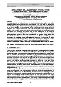
when a model is available for the object, but the parameters that define the model, such as material properties or geometry, are not known or are known to a low certainty. For all three of these cases a trainable neural network model approach to VBFM is preferable. Figure 1 illustrates our neural network modeling approach to VBFM. A sequence of images is taken under various loading conditions. This sequence of images is then passed to the neural network training algorithm. Once the neural network model is trained, it can then be used to measure forces from new images.
This paper presents a method to model the deformation of an elastic object with an artificial neural network. The neural network is trained directly from images of the elastic object deforming under known loads. Using this process, models can be created for objects such as biological tissues that cannot be modeled by existing techniques. The neural network elastic model is used in conjunction with a deformable template matching algorithm to perform vision-based force measurement (VBFM). We demonstrate this learning method on objects with both linear and nonlinear elastic properties.
2. Neural Network Elastic Material Model
1. Introduction
Feed-forward two layer neural networks with the layout shown in Figure 2 are used. Each hidden node has a logistic sigmoid activation function of the form
The ability to manipulate deformable objects has many important application areas particularly in the bioengineering and biomedical domains. Examples include the manipulation of biological cells and robotic surgery. When manipulating deformable objects, it is often useful to have knowledge of the force applied to the object in order to prevent damage. If vision feedback is available for observing object deformations, this feedback can be used to estimate the force applied to these objects. This technique is referred to as vision-based force measurement (VBFM). It has been shown that if an accurate model is available that defines the elastic behavior of an object, then the force applied to that object can be measured using computer vision [2][10]. Three cases exist in which this explicit model based approach is not appropriate. The first case is for materials that exhibit nonlinear elastic properties in which it is computationally prohibitive to calculate the model in realtime. This situation occurs when there are large deflections or the stress-strain relationship for the material is nonlinear. A second case occurs when an accurate material model is unavailable for an object. Some examples are biological structures such as cells and organs. The third situation is 0-7803-7860-1/03/$17.00 © 2003 IEEE
g(a) =
1 1 + exp(−a)
(1)
where a is the sum of all of the weighted inputs to the node. The output nodes have a linear activation function that returns the sum of all of the node’s weighted inputs. The neural network is represented in equation form by
yi = wiP +1 +
P X j=1
" Ã
g vjD+1 +
D X
k=1
!
[vjk xk ] wij
#
(2)
where the neural network has D inputs, P hidden nodes, and N outputs. The hidden layer weights are stored in the v matrix and the output layer weights are stored in the w matrix. Neural networks of this type have the property that they are universal approximators, meaning that the neural network can approximate a general nonlinear function to arbitrary accuracy provided that there are a sufficient number of hidden nodes [6]. 1278 1
Training Data Pairs Images
New Image
Applied Loads 0 mN
40 mN Learning Algorithm
Trained Force Sensor
Force Reading 35 mN 90 mN
Figure 1: Diagram illustrating the learning approach to vision-based force measurement.
Neural Network Elastic Object Model
Hidden Nodes w 11
v11
Inputs v12 x1
w 21
x
y’
F
x2 1
x’
Neural Network
y
Outputs y1
F
(x,y)
v2D+1
Bias Nodes
(x’,y’)
y2 1
w 2P+1
Undeformed Object
Deformed Object
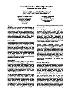
Figure 3: Process of using a neural network elastic model to calculate an object’s deformation due to an applied load F.
Figure 2: Neural network diagram.
The neural network elastic model presented in this paper inputs a point (x, y) from within the object and the load F applied to the object and returns the deformed location (x0 , y 0 ) of the input point. This process is shown Figure 3 for the two dimensional case. For this case, the neural network has three inputs and two outputs. If more than one load is being applied to the object, additional inputs can be added to the neural network. A neural network model constructed in this manner completely defines the deformation of an elastic object subject to an applied load F.
is represented by a list of 2D vertices Ti and the edge pixels in the current image are represented by the list of 2D vertices Ii . The registration algorithm minimizes the distance squared between the transformed template vertices T0i and the nearest image edge vertices Ii where the template vertices are transformed by an elastic transformation and a rigid body transformation.
3.1. The Rigid Body Portion of the Template Matching Algorithm
3. Neural Network Based Deformable Template Matching Algorithm
The rigid body portion of the transformation of the template vertices is simply an affine transformation given by
In order for the neural network elastic model to be useful for computer vision applications, it must be incorporated into a deformable template matching algorithm. The deformable template models both the rigid body portion of an object’s motion and the object’s deformation due to applied loads. The deformable template is registered to a binary edge image [1] using a least square error measure. The template
T0i = A(Ti )
(3)
A is defined by A(T) = X +
·
cos θ sin θ
− sin θ cos θ
¸
T
(4)
where θ is the angle of rotation and X is the translation vector. The error function between the transformed tem1279 2
plate vertices T0i and the image vertices Ii can be written as E(θ, X) =
M X ° 0 ° ° Tj − I j ° 2
the same point in the deformed body. Therefore, in order to train the neural network, it is necessary to obtain training pairs that consist of the x-y coordinate of a point in the undeformed body and the force applied to the body and the x-y coordinate of the same point in the deformed body. Many such points are needed to adequately train the neural network. These training pairs also need to be obtained for many force values over the range of expected loads.
(5)
j=1
where T0j is the position vector of the ith edge pixel of the template transformed by (3); Ij is the position vector of the edge pixel in the image that is closest to the point T0j ; and M is the number of edge pixels in the template. This error function sums the square of the distance between each template vertex and the nearest image edge pixel. Since the transformed template vertices T0j were transformed by the affine transform A, E will be a function of θ and X. By minimizing E, the values of θ and X that best match the image in a least squares sense will be found. The error function E is minimized by a gradient-based multi-variable minimization technique called the BroydonFletcher-Goldfarb-Shanno (BFGS) method [9].
3.2.
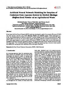
4.1. Obtaining Training Data The training data pairs are obtained directly from images of the object under known loads. Using this approach, a neural network model of the object is created without using an explicit material model for the object. A computer vision algorithm is required that can measure the displacement of a point within an elastic body. A deformable body tracking algorithm is used for this purpose. There are many available deformable body tracking algorithms [4][7][12]. In order for a tracking algorithm to be useful for acquiring training data, it must be invariant to rigid body motions and it must provide a unique tracking solution. Many of the available deformable body tracking algorithms cannot be used here because they do not provide the ability to uniquely determine where a given point moves within a body. Active contour models (snakes) [5] provide a way to track deformable objects but they do not provide a way to uniquely determine where a point in an object moves in a subsequent image. Snakes also have the problem that the rigid body motions are not separated from the deformation of the object. The non-uniqueness problem occurs because the snakes algorithm is not based on an actual material model. A unique tracking solution can be obtained if we use a deformable object tracking algorithm that has knowledge of how materials deform. Two approaches that make use of material models include finite element method (FEM) based algorithms [7] and boundary element method (BEM) based algorithms [3]. We use the BEM deformable body tracking algorithm described in [3], because this algorithm is invariant to rigid body motions and provides a unique solution to the deformable body tracking problem. The BEM method differs from the FEM method in the way the body is partitioned to solve the partial differential equations that define the elasticity problem. For the FEM method the entire domain that defines the object is partitioned into elements (see Figure 4). The BEM method only requires that the boundary of the object is partitioned. Because the BEM method only partitions the boundary of the object, it is more natural for use in computer vision problems where the boundary of the object is often all that is visible. Because the BEM deformable object tracking algorithm makes use of the equations of elasticity, it tracks a deformable contour uniquely. The left half of Figure 5
Incorporating Deformations into the Template Matching Algorithm
Minimizing (5) determines the rigid body motion of the object. We would also like to determine the non-rigid portion of the object’s motion. To do this, the template is deformed according to the neural network elastic model before performing the affine transformation. The transformation becomes T0 = A (N euralN etwork(T, F ))
(6)
where N euralN etwork(T, F ) represents the neural network material model which returns the displaced location for the template edge pixel T due to the applied force F on the object. The error function (5) becomes E(θ, X, F ) =
M X i=1
kT0i − Ii k
2
(7)
Since the error function (6) has an additional parameter F , minimizing the error function gives the applied force F in addition to the position and orientation of the object. This algorithm tracks the deformable object by finding the applied force F that, when applied to the template, causes the template to match the image.
4. Acquisition of Training Data and Network Training As previously shown, the neural network elastic model has three inputs and two outputs. The inputs are the x-y coordinates of a point in the undeformed body and the applied load on the body. The outputs are the x-y coordinates of 1280 3
250 200
Undeformed 0.613 N Load 1.222 N Load
150 100
BEM Mesh
50
FEM Mesh
0
Figure 4: FEM and BEM meshes for a two dimensional object.
−50 −100 −150 −200 −250 −300
−200
−100
0
100
200
300
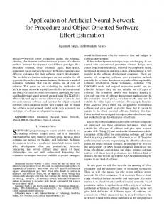
Figure 6: Training data obtained for the rubber torus object under two different applied loads.
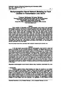
Figure 5: BEM deformable tracking algorithm tracking the rubber torus object. Undeformed template on left and template fitted to deformed torus on right.
shows a deformed rubber torus under a known load along with an undeformed BEM deformable object template. The right half of this figure shows the BEM template matched to the deformed rubber torus. This process is repeated for all of the images used to train the neural network elastic model. The training images should represent the range of loads that are likely to be encountered by the object. Figure 6 shows the training data obtained using the BEM tracking algorithm for the rubber torus object. In the figure, the same edge points are shown for the undeformed torus, the torus under a 0.613 N load and the torus under a 1.222 N load. When these point deformations are obtained for a sufficient number of different loads, they are used to train the neural network elastic model.
Figure 7: Rubber torus loading condition.
well but it may be very inaccurate for loads that were not part of the training data. This last phenomenon is known as over-fitting [6]. In general, the more training pairs that can be used the more accurate the model. The number of hidden nodes used should be the minimum number that still achieves adequate training.
4.2. Training the Neural Network
5. Experimental Results
The neural network is trained using the error backpropagation method [6]. The success of the training process depends on the number of training pairs that are used and the number of hidden nodes in the neural network model. If there are not a sufficient number of training data pairs, the network may model the training data well, but it will not be able to perform well for new loads that were not part of the training data. Also, if there are not a sufficient number of hidden nodes, the neural network will not be able to model the elastic object to a high degree of accuracy. However, if there are too many hidden nodes, the neural network will be able to model the training pairs very
5.1. Rubber Torus Application The neural network elastic model was first applied to the rubber torus object shown in Figure 5 with a force applied as shown in Figure 7. The torus, because it is constructed of rubber, has nonlinear elastic behavior. Therefore, it is computationally infeasible to model the elastic behavior of this object accurately in real-time. A neural network was trained directly from 39 images of the torus under loads between 0 and 0.84 N. There were 70 hidden nodes in the neural network model. Once the training process was com1281 4
Figure 10: Microgripper. Figure 8: Neural network based deformable tracking algorithm tracking the rubber torus object. Undeformed template on left and template fitted to deformed torus on right. 0.9
Load Measured by Vision Algorithm (N)
0.8
Vision Algorithm Actual Force
0.7
Figure 11: Experimental setup for measuring microgripper gripping force.
0.6 0.5
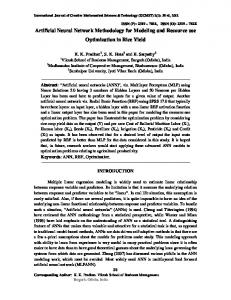
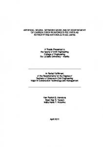
VBFM was applied to this gripper by modeling each jaw of the microgripper as a cantilever beam [2]. This model based approach required precise knowledge of the material properties and geometric parameters of the microgripper. It also required a precise calibration of the camera system so that deflections in pixel space can be converted into world space deflections. The experimental setup shown in Figure 11 makes use of a piezoresistive force sensor to measure the clamping force for the microgripper. Figure 12 shows a plot of force versus clamping tube position comparing the cantilever beam model based VBFM method to the piezoresistive force sensor. The average error with this model based approach was 6.0 mN. The neural network modeling approach can be applied to the microgripper avoiding the need for precise knowledge about the parameters that define the microgripper or precise camera calibration. Figure 13 shows a plot of force versus tube position comparing the neural network based force measurement to the piezoresistive force sensor. The average error is 3.4 mN. Not only does the neural network modeling approach avoid having to model the microgripper, but it also provides a more accurate result. The neural network approach is more accurate in this case because it is not necessary to assume values for the material properties and geometry of the microgripper.
0.4 0.3 0.2 0.1 0.1
0.2
0.3
0.4 0.5 0.6 Applied Load (N)
0.7
0.8
0.9
Figure 9: Neural network elastic model force measurement results for the rubber torus object.
pleted, the neural network elastic model was used to predict the force applied to the object visually as shown in Figure 8. This figure shows the torus being tracked with the deformable template based on the neural network model. This trained model was applied to 39 images that were not used in the training process. Figure 9 shows a plot of vision-based force measurement versus applied load. The average error in the vision-based force measurement was 10.7 mN.
5.2. Microgripper Application The neural network modeling method was also applied to the microgripper shown in Figure 10. The microgripper was cut by micro-wire EDM from spring steel 254 microns thick. A tube is slid over the microgripper to force the jaws of the gripper together in order to grasp an object [11]. When this microgripper is used for a microassembly task it is important to measure the gripping force that the microgripper applies to the object being held. Previously,
6. Conclusions We have presented a method to model the deformation of elastic objects through the use of artificial neural networks. The neural network model can be incorporated into a deformable template matching algorithm to perform vision1282 5
0.14 0.12
0.14 Piezoresistive Sensor Cantilever Model VBFM
0.12 0.1
Clamping Force (N)
Clamping Force (N)
0.1 0.08 0.06
0.08 0.06
0.04
0.04
0.02
0.02
0 0
Piezoresistive Sensor Neural Network VBFM
0.5
Tube Position (mm)
1
0 0
1.5
0.5
Tube Position (mm)
1
1.5
Figure 12: Cantilever beam model based VBFM results for microgripper showing an average error of 6.0 mN.
Figure 13: Neural network model based VBFM results for microgripper showing an average error of 3.4 mN.
based force measurements. This technique is useful for objects that have complex material models or that can not be accurately modeled with existing modeling techniques. It was also shown that this method can be useful even when there is an available model for the object because the neural network based method does not require knowledge of material properties or geometry. A precisely calibrated camera system is also not needed with the neural network approach. This learning by seeing method is particularly useful for the manipulation of biological tissues or cells because it is difficult to accurately model such objects. These objects also tend to be easily damaged if excessive loads are applied, making force feedback essential.
[3] Greminger, M.A., Nelson, B.J., “Deformable Object Tracking Using the Boundary Element Method,” IEEE Conference on Computer Vision and Pattern Recognition (CVPR2003),June 2003. [4] Jain, A. K., Zhong, Y., Dubuisson-Jolly, M.P., “Deformable template models: A review,” Signal Processing, Vol. 71, pp. 109-129, 1998. [5] Kass, M., Witkin, A., Terzopoulos, D., “Snakes: Active Contour Models,” International Journal of Computer Vision,pp. 321-331, 1988. [6] Kecman, V., Learning and Soft Computing, MIT Press, Cambridge, Mass, 2001. [7] Metaxas, D., Physics-Based Deformable Models, Kluwer Academic Publishers, Boston, Mass, 1997. [8] Tsap, L., Goldgof, D., Sarkar, S., “Efficient Nonlinear Finite Element Modeling of Nonrigid Objects via Optimization of Mesh Models,” Computer Vision and Image Understanding, Vol. 69, pp. 330-350, March 1998. [9] Vanderplaats, G., Numerical Optimization Techniques for Engineering Design, McGraw-Hill, New York, 1984. [10] Wang, X., Ananthasuresh, G. K., Ostrowski, J. P., “Visionbased sensing of forces in elastic objects,” Sensors & Actuators A-Physical, Vol. 94, No. 3, pp. 142-156, November 2001. [11] Yang, G., Gaines, J. A., Nelson, B. J., “A Flexible Experimental Workcell for Efficient and Reliable Wafer-Level 3D Microassembly,” Proc. 2001 IEEE Int. Conf. of Robotics and Automation (ICRA2001), Soul, Korea, May 2001. [12] Yuille, A., Cohen, D., Hallinan, W., “Feature extraction from faces using deformable templates,” International Journal of Computer Vision, Vol. 8, No. 2, pp. 99-111, 1992.
Acknowledgments This research was supported in part by the National Science Foundation through Grant Numbers IIS-9996061 and IIS-0208564. Michael Greminger is supported by the Computational Science Graduate Fellowship (CSGF) from the Department of Energy.
References [1] Canny, J., “A Computational Approach to Edge Detection,” IEEE Transactions on Pattern Analysis and Machine Intelligence,Vol. PAMI-8, No. 6, November 1986. [2] Greminger, M.A., Yang, G., Nelson, B.J., ”Sensing nanonewton level forces by visually tracking structural deformations,” IEEE Int. Conf. on Robotics and Automation (ICRA2002), May, 2002.
1283 6