Neural Network for LIDAR detection of fish Vikramjit Mitra1 Chia-Jiu Wang2 George Edwards1 Email:
[email protected],
[email protected],
[email protected] 1 University of Denver, Department of Engineering, Denver, CO 2 University of Colorado at Colorado Springs, ECE department Colorado Springs, CO 80933 neural network for classification of under water fish, water layer and water bed from airborne LIDAR data. The difference in the pattern of the LIDAR backscatter when there is a fish shoal underneath the water and when there is an underlying bottom close to the water surface enables us to classify the different cases by analyzing the reflected pattern. The network is trained by the features extracted from the backscatter and these features are used to distinguish between the different cases, so that the main target of the network is feature detection. The airborne LIDAR data studied in this paper are obtained from National Oceanic and Atmospheric Administration (NOAA), Colorado.
Abstract In this paper we present a neural network for detection of fish, from Light Detection And Ranging (LIDAR) data and have described a classification method for distinguishing between water-layer, bottom and fish. Four multi-layer perceptrons (MLP) were developed for the classification purpose, where classes include fish, bottom and waterlayer. The LIDAR data gives a sequence of intensity of laser backscatters obtained from laser shots at various heights above the earth surface. The data is preprocessed to remove the high frequency noise and then a window of the sample is selected for further processing to extract features for classification purpose. We have used Linear Predictive Coding (LPC) analysis for the feature detection purpose. The results show that the detection technique is effective and can do the required classification with a high degree of accuracy. We have tried our approach with four different MLPs and are presenting the data obtained from each of them.
1.1 The LIDAR All LIDAR systems operate on the principle that water depth may be calculated from the time difference between laser returns reflected from the sea surface and seabed. Commonly, an infrared channel (1064 nm) is used for surface detection, while bottom detection is from a bluegreen channel [3]. The process of gathering LIDAR data is discussed briefly here. The basic geometry of how the laser shots are taken is shown in Figure 1.1a. The ideal response of the LIDAR reflection is shown in Figure 1.1b.
1. Introduction Classification of remote objects through LIDAR technique has been of intensive investigation these years [1,2,3]. It is advantageous mainly due to high area coverage coupled with high spatial data density, rapid response and cost effectiveness [4]. A LIDAR transmits and receives electromagnetic radiation at a high frequency and operates in the ultraviolet, visible and infrared region. The LIDAR instrument transmits light out to a target. The transmitted light interacts with and is changed by the target. Some of this light is reflected and scattered back to the instrument where it is analyzed. The change in the properties of the light enables us to determine some properties of the target. The time for the light to travel to the target and back to the LIDAR is used to determine the range of the target. Classification of remote objects through neural networks from LIDAR data is advantageous solely due to the intrinsic property of artificial neural networks: efficient classification of data, parallel computation potentials, high adaptivity and great error tolerance [6]. In this paper, we present the results of using multi-layer perceptron (MLP) -------------------The authors would like to acknowledge NOAA for providing the real experimental data. 0-7803-7898-9/03/$17.00 ©2003 IEEE
Fig 1.1a. LIDAR shots taken [3] The LIDAR back scatter is plotted as amplitude of back scatter versus time, the LIDAR shots are taken from an airborne object as shown in Fig: 1.1a.
1001
depicts the intensity of the back scatter of the laser shot at various distances from the airborne object.
Fig 1.1b. Back scatter of LIDAR (Y- Amplitude of backscatter, X- Time after the LIDAR shot) [3].
Fig 1.1d. LIDAR Back scatter for water layer (YAmplitude of backscatter, X- Time after the LIDAR shot).
Figure 1.1b shows the plot of the intensity of back scatter versus time for one laser shot. First the LIDAR shot has to traverse through the atmosphere. Due to lack of reflecting particles, the amplitude of reflection is minimun here, as shown in Figure 1.1b. But one may get some reflection due to presence of fog in atmosphere. As the LIDAR shot moves down towards earth surface it first hits the water surface, here at air-water interface, due to change in the density of the medium we get a huge amount of reflection that results in obtaining a peak in the backscatter plot, as shown in Figure 1.1b. As the LIDAR beam penetrates water three cases might arise: (1) Presence of water layer only (Fig 1.1d), without any object from where we can have any reflection, in this case the amplitude of backscatter falls sharply as the laser penetrates the depths of the water and finally dies. (2) Presence of some under water object (Fig 1.1d) from where some LIDAR backscatter happens. (3) Presence of a bottom, from where we obtain a high amount of backscatter (Fig 1.1f) thus creating an immideate peak after the water surface peak.
Fig 1.1d depicts characteristics of the LIDAR shot in case of water layer. The peak represents the interface between air and water which results in a huge reflection of the laser beam. The reflection dies steadily as we penetrate deeper into the water.
Fig 1.1e. LIDAR Backscatter for fish (Y- Amplitude of backscatter, X- Time after the LIDAR shot). As the laser traverses to the depths of water, we may find some more stray reflections as pointed in Figure 1.1e which implies that there might be some object underneath, that resulted in that back scatter.
The raw data obtained from NOAA were in form of files and each file contained a set of 2000 LIDAR back scatter information. The intensity of the back scatter when plotted gives the Fig 1.1c, where the horizontal axis depicts the total number of laser shots present in the file. 100 200 300 400 500 600 700 800 900 1000
200
400
600
800
1000
1200
1400
1600
1800
2000
Fig 1.1c. Plot of LIDAR backscatter (Y- Time after the LIDAR shot, X- Number of LIDAR shots)
Fig 1.1f. LIDAR Backscatter for bottom (Y- Amplitude of backscatter, X- Time after the LIDAR shot).
The wavy intensity spectrum suggests that the airborne object was moving and hence the distance between that and water surface was changining. The spectrum actually
Figure 1.1f depicts the presence of a water bed close to the water surface, which produces a good amount of back 1002
scatter. In this case there are two interfaces, air-water interface and water-bottom inteface, which results in two peaks as evident from the Fig 1.1e.
coefficients, fewer bits are needed to transfer the sample. Compression is achieved by building a predictive model of the waveform [7]. The predictive coefficients obtained from LPC coding are a linear combination of all the previous samples.
Presence of stray reflections from underneath the water surface can have many implications. It may imply that there is fish or phytoplankton colony or algae population . To detect and catergorize each of them, we have to implement different feature detection techiques that might help in classifying them into different classes
Linear predictive coding is an established autoregressive model for a wide variety of waveforms. Here the predicted waveform is a linear combination of past samples as represented by the following equations:
We know that, the plankton population as well as the algae population extends for a wider area, much larger than that of fish. This would result in obtaining under-water object reflections for a longer span than that of fish. Thus, to detect them we have to implement a temporal detection methodology governed by the following rule-based algorithm.
The coded signal, e(t), is the difference between the estimate of the linear predictor ŝ(t), and the speech signal s(t)
If (presence of back scatter reflection below water level) { If (time for that reflection > N) Then (Class = Algae OR Class = Phytoplanktons) Else (Class = Fish).} Else (Class = Other).
However, many waveforms of interest are not stationary. The best values for the coefficients of the predictor, ai, vary from one section of the waveform to another. It is often reasonable to assume that the signal is pseudostationary, i.e. there exists a time-span over which reasonable values for the linear predictor can be found.
The time N can be in minutes or seconds, which we have to set depending upon the optimal value that is possible to detect the desired objects with a certain level of accuracy. Our main purpose is to detect fish in this case and thus we are ignoring the case of phytoplanktons and algae population right now.
2.2 LPC coefficient analysis In this approach, we preprocess the data before obtaining the LPC coefficients. The preprocessing consists of filtering the data using a butter-worth filter to get rid of the high frequency components. These high frequency components add noise to the signal and make the process of feature extraction from the LPC coefficients difficult. After filtering the data, we select the peak value of the backscatter amplitude (which actually gives the air-water interface point) and take a window of 175 points after it. As observed from the LIDAR backscatter plots, Fig 1.1d, 1.1e and 1.1f, the data before the peak value is irrelevant for our case as it is the backscatter data from air and hence does not provide any information about the under water objects. Similarly from our observation we have noticed that the significant information about under water objects is present within the 175 points after the peak value and after this noise comes into play, which again hinders the process of feature extraction. After preprocessing we have broken the data into 10 LPC coefficients. Fig 2.1 shown below is the block diagram for LPC analysis
2. Data Analysis In this section we will analyze some samples and will try to detect some features which will help to classify the different classes. We will apply linear prediction coding technique to analyze the LIDAR data sets. 2.1 Linear Predictive Coding Linear Predictive Coding (LPC) is a predominant method that breaks a signal into specific characteristics and encodes just these characteristics rather than the whole sample. This is mainly used for speech signals. LPC uses the fact that every sound has unique attributes, i.e. frequency, resonance, loudness etc. By breaking each sample down into these components to generate prediction
1003
The data is encoded into LPC coefficients and our main task is to detect the features from these LPC coefficients, so that we can categorize between the three classes. Figure 2.1 shows the block diagram of LPC analysis, which depicts the flow diagram of preprocessing the data and then taking LPC coefficients of the same. The LPC coefficients thus obtained are used to train the neural network. We have broken each data into 10 LPC, thus corresponding to each data we have 10 coefficients = {a0, a1, a2, a3, a4, a5, a6, a7, a8, a9 }. From our observation we have found that a0 is always 1 for all the cases, and this introduces a confusion for the network to draw a strong decission boundery. Due to this, we have ignored a0 for trainig purpose and now we are left with the remaining 9 coefficients to train the neural network.
0.2
0
-0.2
-0.4
-0.6
-0.8
-1
-1.2
2
3
4
5
6
7
8
9
Fig 2.4 LPC values vs coefficient numbers (for bottom) (Y- LPC Value, X-Number of LPC coefficients) The figure 2.4 depicts the case for bottom, here the coefficient a1 goes to approximately -1 value as usual, but the other coefficients oscillates along the 0 value. It is also quite distinct that the oscillation is much less than that of the water layer case. Thus, we can see that the LPC coefficients provide us with some features that help us to detect between the three categories.
In this section we will discuss briefly the distinguishing features of the LPC coefficient for the three different categories – fish, water-layer and water-bottom. 0.4
0.2
3. Artificial Neural Networks
0
-0.2
Artificial Neural Networks (ANN) are distributed, adaptive, generally nonlinear learning machines built from many different processing elements (PEs) [5]. Each PE receives connections from other PEs and/or itself. The interconnectivity defines the topology. The signals flowing on the connections are scaled by adjustable parameters called weights, wij. The PE’s sum all these contributions and produce an output that is a nonlinear (static) function of the sum. The PE’s outputs become either system outputs or are sent to the same or other PE’s. Figure 3 shows as an example of an ANN.
-0.4
-0.6
-0.8
-1
1
1
2
3
4
5
6
7
8
9
Figure 2.2 LPC coefficients for fish (Y- LPC Value, X-Number of LPC coefficients) Figure 2.2 depicts the LPC coefficients corresponding to fish data. Here we observe that the a1 coefficient value falls to -1 and then it remains steadily close to 0 values for all the other coefficients. There is little or no oscillation of the value for the other coefficients and they remain almost a constant and approximately zero. 0.4
0.2
0
-0.2
-0.4
Fig 3.1 An Artificial Neural Network
-0.6
In this research, we have employed multilayer perceptrons (MLPs) with different number of hidden layers. The number of Processing Elements (PE) may vary for each layer. We have implemented two approaches to optimize the output and have studied the behavior of the neural network in these two cases. The basic flow diagram of the neural network and the decision logic is shown in fig 3.2. The MLP has 9-input nodes, corresponding to the 9 LPC coefficients. We have considered two cases for the output nodes: 1-output node and 2-output node. We have used sigmoid as the activation function.
-0.8
-1
1
2
3
4
5
6
7
8
9
Fig 2.3 LPC values vs coefficient numbers for water layer (Y- LPC Value, X-Number of LPC coefficients) The figure 2.3 represents the LPC coefficient plot for water layer. Here we can see that for coefficient a1 the value goes down to -1 as before, but later for the other coefficients, it oscillates along the 0 value, which is quite distinct than that of the case of the fish. 1004
9-Input 1-Output MLP Output Desired Actual After decision logic 1.0 0.8393 1.0 1.0 0.5892 0.5 1.0 0.7832 1.0 0.5 0.3175 0.5 0.5 0.3045 0.5 0.5 0.2859 0.5 0.0 0.0056 0.0 0.0 0.0019 0.0 0.0 0.0026 0.0 Table 4.1 MLP with one hidden layer
Fig 3.2 Neural network with decision logic module. 1-Output: Rule-based decision is used here and the results are quantified as fish = 1, water = 0.5 and bottom = 0. Desired output 1 0.5 0 Implication Fish Layer Bottom Table 3.1 Desired output for 1-output case.
Output Desired Actual After decision logic 1.0 0.8879 1.0 1.0 0.5734 0.5 1.0 0.7671 1.0 0.5 0.3376 0.5 0.5 0.3155 0.5 0.5 0.2662 0.5 0.0 0.0179 0.0 0.0 0.0118 0.0 0.0 0.0122 0.0 Table 4.2 MLP with two hidden layers
2-Output: Here also rule based decision is incorporated and the results are quantified fish = 1 0, water-layer = 0 1 and bottom = 0 0. Desired output 1 0 0 1 0 0 Implication Fish Layer Bottom Table 3.2 Desired output for 2-output case. The network is constructed using the software Neurosolution Wizard Version3 [5]. The outputs from the neural network is expected to have values corresponding to table 3.1 (for 1-output) and 3.2 (for 2-output), but the actual outputs are close to these values but not exactly equal to them. To make a clear decision, we have used a decision logic module (fig 3.2), which has a decision boundary that helps to make the final decision (Table 3.3 and 3.4).
Output Desired Actual After decision logic 1.0 0.8630 1.0 1.0 0.5431 0.5 1.0 0.7321 1.0 0.5 0.2115 0.0 0.5 0.3799 0.5 0.5 0.2601 0.5 0.0 0.0711 0.0 0.0 0.0704 0.0 0.0 0.0781 0.0 Table 4.3 MLP with three hidden layers
Decision boundary Upper Lower Fish < = 1.0 > 0.75 Layer < = 0.75 > 0.25 Bottom < = 0.25 > = 0.0 Table 3.3 Decision boundary for 1-output node Decision boundary Node-1 Node-2 Upper Lower Upper Lower Fish < = 1.0 > = 0.5 < 0.5 > = 0.0 Layer < 0.5 > = 0.0 < = 1.0 > = 0.5 Bottom < 0.5 > = 0.0 < 0.5 > = 0.0 Table 3.4 Decision boundary for 2-output node
Output Desired Actual After decision logic 1.0 0.8883 1.0 1.0 0.5687 0.5 1.0 0.7671 1.0 0.5 0.2765 0.5 0.5 0.3797 0.5 0.5 0.2635 0.5 0.0 0.0753 0.0 0.0 0.0755 0.0 0.0 0.0734 0.0 Table 4.4 MLP with four hidden layers
4. Results and Discussions We have considered 9-input 1-output and 9-input 2-output neural network. The results obtained from 9-input 1-output Neural network are presented below. We have used 60 samples to train the network (20 samples from each category) and 9 samples to test the network.
1005
three classes were very close to each other without any strong decision plane separating the classes, but despite this the network is found to be working efficiently. The final decision is inferred by using rule based decision logic. A better approach would be to fuzzy logic module to do the inferencing. As the LIDAR samples for fish and water-layer is very close to each other, hence extracting features to distinguish between them was the major for our case. We have also tried to use slope analysis for feature detection, but so far LPC analysis gave the best result and accuracy. Another better way would be to use Linear Predictive Coding (LPC) with Fast Fourier Transform (FFT) to extract the features from LIDAR data, which can yield promising results with high accuracy. As the output of the neural network is in form of numbers, which closely resembles fuzzy membership functions, hence the best possible solution would be to implement a neural-fuzzy approach.
9-Input 2-Output MLP Desired 1 0 1 0 1 0 0 1 0 1 0 1 0 0 0 0 0 0
Actual After decision logic 0.9565 0.0172 1 0 0.9661 0.0334 1 0 0.9225 0.0251 1 0 0.0119 0.6178 0 1 0.0223 0.7568 0 1 0.0236 0.5123 0 1 0.0432 0.0001 0 0 0.0022 0.0113 0 0 0.0524 0.0025 0 0 Table 4.5 MLP with one hidden layer
Desired 1 0 1 0 1 0 0 1 0 1 0 1 0 0 0 0 0 0
Actual After decision logic 0.9364 0.0371 1 0 0.9160 0.0428 1 0 0.9119 0.0226 1 0 0.0217 0.5084 0 1 0.0281 0.6698 0 1 0.0315 0.5021 0 1 0.0628 0.0002 0 0 0.0030 0.0128 0 0 0.0045 0.0119 0 0 Table 4.6 MLP with two hidden layers
Desired 1 0 1 0 1 0 0 1 0 1 0 1 0 0 0 0 0 0
Actual After decision logic 0.9488 0.0357 1 0 0.9418 0.0414 1 0 0.9445 0.0339 1 0 0.1764 0.7968 0 1 0.0912 0.9014 0 1 0.0856 0.9001 0 1 0.0072 0.0112 0 0 0.0705 0.0114 0 0 0.0088 0.0011 0 0 Table 4.7 MLP with three hidden layers
Desired 1 0 1 0 1 0 0 1 0 1 0 1 0 0 0 0 0 0
References [1] Professor R. Sica, Department of Physics and Astronomy, University of Western Ontario, “Exploring the Atmosphere With Lidars” http://pcl.physics.uwo.ca/pclhtml/introlidar/introlidarf.html [2] Dr. James E. Arnold, Dr. Michael J. Kavaya, NASA “LIDAR Tutorial” http://www.ghcc.msfc.nasa.gov/sparcle/sparcle_tutorial.ht ml [3] Geraint R. West, W. Jeff Lillycrop, Joint Airborne Lidar Bathymetry Technical Center of Expertise, AL. “Feature Detection and Classification with Airborne Lidar- Practical Experience” http://shoals.sam.usace.army.mil/pdf/West_Lillycrop_99.p df. [4] Guenther, G.C., T..J. Eisler, J.L. Riley, and S.W. Perez, 1996. “Obstruction detection and data decimation for airborne laser hydrography,” Proc. 1996 Canadian Hydro. Conf., June 3-5, Halifax, N.S.
Actual After decision logic 0.9310 0.0084 1 0 0.9429 0.0071 1 0 0.9511 0.0069 1 0 0.0961 0.3905 0 0 0.0102 0.9030 0 1 0.0101 0.6711 0 1 0.1494 0.0568 0 0 0.1061 0.0750 0 0 0.0989 0.0566 0 0 Table 4.8 MLP with four hidden layers
[5] Principe, Euliano, Lefebvre "Neural and Adaptive Systems: Fundamentals Through Simulations" John Wiley & Sons, Inc. 2000. [6] Rongrui Xiao, Robert Wilson and Richard Carande. Vexcel Corporation, 4909 Nautilus Ct., Suite 133, Boulder CO 80301. “Neural Network Classification with IFSAR and Multispectral Data Fusion” 1998 IEEE trans http://www.vexcel.com/papers/nn_class.pdf
From the results obtained above it is evident that the neural network works efficiently in detecting the required classes. We have considered LPC coefficients as data, as evident from the data analysis, the LPC coefficients for all the
[7] N. S. Jayant, P. Noll, “Digital Coding Of Waweforms” Prentice-Hall Signal Processing Series. Prentice-Hall, Inc., 1984. 1006