Atmos. Chem. Phys. Discuss., 4, 3653–3667, 2004 www.atmos-chem-phys.org/acpd/4/3653/ SRef-ID: 1680-7375/acpd/2004-4-3653 © European Geosciences Union 2004
Atmospheric Chemistry and Physics Discussions
ACPD 4, 3653–3667, 2004
Neural networks and tracer correlations D. J. Lary and H. Y. Mussa
Using an extended Kalman filter learning algorithm for feed-forward neural networks to describe tracer correlations D. J. Lary1, 2, 3 and H. Y. Mussa3
Title Page Abstract
Introduction
Conclusions
References
Tables
Figures
J
I
J
I
Back
Close
1
Global Modelling and Assimilation Office, NASA Goddard Space Flight Center, USA GEST at the University of Maryland Baltimore County, MD, USA 3 Unilever Cambridge Centre, Department of Chemistry, University of Cambridge, United Kingdom 2
Received: 19 April 2004 – Accepted: 21 June 2004 – Published: 30 June 2004 Correspondence to: D. J. Lary (
[email protected])
Full Screen / Esc
Print Version Interactive Discussion
© EGU 2004 3653
Abstract
5
10
15
20
25
ACPD
In this study a new extended Kalman filter (EKF) learning algorithm for feed-forward neural networks (FFN) is used. With the EKF approach, the training of the FFN can be seen as state estimation for a non-linear stationary process. The EKF method gives excellent convergence performances provided that there is enough computer core memory and that the machine precision is high. Neural networks are ideally suited to describe the spatial and temporal dependence of tracer-tracer correlations. The neural network performs well even in regions where the correlations are less compact and normally a family of correlation curves would be required. For example, the CH4 -N2 O correlation can be well described using a neural network trained with the latitude, pressure, time of year, and CH4 volume mixing ratio (v.m.r.). The neural network was able to reproduce the CH4 -N2 O correlation with a correlation coefficient between simulated and training values of 0.9997. The neural network Fortran code used is available for download.
4, 3653–3667, 2004
Neural networks and tracer correlations D. J. Lary and H. Y. Mussa
Title Page Abstract
Introduction
Conclusions
References
Tables
Figures
J
I
J
I
Back
Close
1. Introduction Compact correlations between long-lived species are well-observed features in the middle atmosphere, as for example described by Fahey et al. (1989); Plumb and Ko (1992); Loewenstein et al. (1993); Elkins et al. (1996); Keim et al. (1997); Michelson et al. (1998); Rinsland et al. (1999); Strahan (1999); Fischer et al. (2000); Muscari et al. (2003). The correlations exist for all long-lived tracers – not just those which are chemically related. This is due to their all be transported by the general circulation of the atmosphere. The tight relationships between different constituents have led to many analyses where measurements of one tracer are used to infer the abundance of another tracer. These correlations can also be used as a diagnostic of mixing (Schoeberl et al., 1997; Morgenstern et al., 2002) and to distinguish between air-parcels of different origins (Waugh and Funatsu, 2003). The description of such spatially and temporally 3654
Full Screen / Esc
Print Version Interactive Discussion
© EGU 2004
5
dependent correlations are usually achieved by a family of correlations. However, a single neural network is a natural and effective alternative as shown by our previous study (Lary et al., 2004). This study uses the same dataset as Lary et al. (2004) but uses a quicker and more accurate extended Kalman filter learning algorithm for feed-forward neural networks as described in the next section. 2. Extended Kalman filter as a learning algorithm for feed-forward neural network
10
15
20
25
For a general introduction to neural networks please see the book by Bishop (1996). In this study we use a new advanced extended Kalman filter learning algorithm for feedforward neural network. The algorithm used here gave better results in just 3 training epochs (iterations) than our previous study (Lary et al., 2004) using the “JETNET 3.4” package (Lonnblad et al., 1992; Peterson et al., 1994) achieved in 1 million epochs. It is well known now that finding the optimal synaptic weights of feed-forward neural networks (FNN) employing gradient descent optimization techniques is plagued by extraordinarily slow convergence rates and misfittings (Shah et al., 1992; Blank and Brown, 1994). A number of faster and more accurate methods have been suggested (Blank and Brown, 1994; Iiguni et al., 1992; Watrous, 1987) at the expense of higher computational cost at each iteration. The extended Kalman filter (EKF) is the best known among them (Singhal and Wu, 1989). With the EKF approach, the training of the FFN can be seen as state estimation for a non-linear stationary process (Singhal and Wu, 1989). What this means exactly will be explained in details in the following sections. The EKF method gives excellent convergence performances provided that there is enough computer core memory and that the machine precision is high. For a large FNN, the storage requirement can become prohibitive. Furthermore, it was noticed (Bierman, 1977) that round off errors due to poor computer precision can sometimes make the algorithm numerically unstable. 3655
ACPD 4, 3653–3667, 2004
Neural networks and tracer correlations D. J. Lary and H. Y. Mussa
Title Page Abstract
Introduction
Conclusions
References
Tables
Figures
J
I
J
I
Back
Close
Full Screen / Esc
Print Version Interactive Discussion
© EGU 2004
5
10
15
The storage issue has been addressed by a number of research groups (Shah et al., 1992; Puskorius and Feldkamp, 1994). They attacked the estimation problem (training) by partitioning it into a set of subproblems assuming the existence of mutually independent groups of weights; the numerical stability issue can be overcome by using the square root of the estimate error covariance matrix (background error covariance matrix) instead of propagating the full estimate error covariance matrix (Bierman, 1977; Zhang and Li, 1999). It should be, however, noted that only the global (full) EKF is described by Bierman (1977); Zhang and Li (1999). We are not aware of anyone who has combined the partitioning approach with the square root scheme. As our work required neural networks of moderate sizes, we employed the global EKF in conjunction with the square root scheme for training the FNN. In the following section we describe briefly how the EKF can be used as a training technique for the FNN. We also give a comprehensive description of how our training algorithm has been implemented.
– Multilayer feed-forward neural networks can be viewed as a static non-linear dynamic system whose state is the vector containing all its synaptic weights.
25
4, 3653–3667, 2004
Neural networks and tracer correlations D. J. Lary and H. Y. Mussa
Title Page Abstract
Introduction
Conclusions
References
Tables
Figures
J
I
J
I
Back
Close
2.1. Employment of EKF As FNN training algorithm Singhal and Wu (1989) first suggested to use an extended Kalman filter for training neural networks. Their argument was simple and it can be put as follows
20
ACPD
– Therefore the training of the neural networks can be considered as a state estimation problem for a stationary non-linear system. – Furthermore, Kalman filter is known to give an optimal estimate of states of linear dynamic systems. It is also equally well known that an extended version of the Kalman algorithm can be used for estimating the approximate conditional means and covariance of1 of the non-linear dynamic systems. 1
conditional mean and covariance: because the EKF is not an optimal filter.
3656
Full Screen / Esc
Print Version Interactive Discussion
© EGU 2004
– Hence, if the neural network is formulated in terms of space-state concepts similar to those of a static non-linear dynamic system, then the best conditional mean and covariance of the synaptic weight vector can be found by employing an extended Kalman filter. 5
10
In state estimation form, mathematically the neural network can be described by these two equations (Shah et al., 1992; Zhang and Li, 1999; Haykin, 2001). wj +1 = wj + ej
(1)
dj = h[wj , xj ] + νj
(2)
ACPD 4, 3653–3667, 2004
Neural networks and tracer correlations D. J. Lary and H. Y. Mussa
The first equation is known as the process equation, whereas the second equation is called the observation equation. – j is the iterative index. – h[wj , xj ] is the iterative varying function describing the network; the value of the function is the FNN output.
Title Page Abstract
Introduction
Conclusions
References
Tables
Figures
J
I
J
I
Back
Close
– dj is the known output (observed, desired, or target) vector. 15
– νj is the measurement noise vector. – xj is the input vector. – wj is the state (vector elements of which are the synaptic weights) of FNN at j.
Full Screen / Esc
– ej is the process noise vector. 20
The assumptions made are: T νj is a white noise with E [νi νj ] = δi j Rj covariance matrix. T
ej is a white noise with E [ei ej ] = δi j Qj covariance matrix. E [ei νTj ] = 0., for all i,j.
Print Version Interactive Discussion
© EGU 2004 3657
2.2. Training procedure using EKF
5
ACPD
ˆ (the state vector) that The training (state estimation) is now a problem of determining w minimizes the sum of squared prediction errors of all observed data so far. ˆ can be obtained by using the Given dj ,hj ,Rj , and Qj , the EKF solution to finding w following recursion (Haykin, 2001) ˆj =w ˆ j −1 + Kj (dj − yˆ j ) w Kj =
(3)
Pj −1 Hj
Title Page
ˆ j −1 , xj ] ∂h[w
(6)
ˆ j −1 ∂w
2.3. Computational aspects 15
20
D. J. Lary and H. Y. Mussa
(5)
Kj is the Kalman gain matrix at step j ; dj − yˆ j vector contains the prediction errors (innovations); yˆ j is the prediction (=h[wj −1 , xj ]); Pj is the estimate of conditional mean covariance matrix; Hj is a matrix of derivatives of hj with respect to all elements of ˆ j −1 w Hj =
Neural networks and tracer correlations
(4)
Rj + HTj Pj −1 Hj
Pj = Pj −1 − Kj HTj Pj −1 + Qj
10
4, 3653–3667, 2004
Consider a neural network with an architecture with one input layer containing n nodes plus one offset node, one hidden layer with m number of nodes plus one offset node, and l number of output nodes in the output layer. In this architecture w is a [m(n+1)+ m+1]×l vector ; x is (n+1) where x(1) is a constant ; P and Q are l[m(n+1)+ m+1]× l[m(n+1)+ m+1] ; R and dj are l×l ; K is [m(n+1)+ m+1]×l ; H is l[m(n+1)+ m+1]×l[m(n+1)+ m+1]. 3658
Abstract
Introduction
Conclusions
References
Tables
Figures
J
I
J
I
Back
Close
Full Screen / Esc
Print Version Interactive Discussion
© EGU 2004
5
For the training procedure to work, it requires values of Pj , Rj , and Qj . Rj is just the error covariance of the observation ( the known data ) so it is easy to calculate. Qj is usually set to zero. However, P is not known a priori. So it is initialized at the beginning of the training. Also w is initialized. The training procedure is implemented as follows 1. Initializations – Choose random values for w0 – Set the offsets (biases) to nonzero constants.
ACPD 4, 3653–3667, 2004
Neural networks and tracer correlations D. J. Lary and H. Y. Mussa
– Initialise P0 to a small nonzero number. 10
2. Choose an input training pattern, xj , which is propagated through the network to yield an output. 3. Rj – If the errors of the input pattern are known, calculate Rj .
Title Page Abstract
Introduction
Conclusions
References
Tables
Figures
J
I
J
I
Back
Close
– If not, use iteration-varying forgetting factor in its place (Zhang and Li, 1999). 15
4. Compute Hj 5. Calculate Kj 6. Update Full Screen / Esc
ˆ j by using the Kalman matrix and the innovations. – w – Pj as shown in Eq. (5). 20
Print Version
7. If the stopping criteria is met, exit. Otherwise go back to step 2. For full details of the process see Sect. 2 in Haykin (2001). In this work: 3659
Interactive Discussion
© EGU 2004
– The FNN had only one output, i.e. dj , Rj , the innovation and the denominator in Eq. (3) are all scalars.
5
– yˆ j = h(w, x) = tanh[w(m(n + 1) + 1 : m + 1)T z(1 : m + 1)], where z(2 : m + 1) = tanh[w(1 : n + 1)T x(1 : n + 1)] and x(1) and z(1) are the biases in the input and hidden layers respectively – Qj = 0.0
4, 3653–3667, 2004
Neural networks and tracer correlations D. J. Lary and H. Y. Mussa
– Rj = Iλj , where λj is a forgetting factor given by Zhang and Li (1999): λj = λ0 λj −1 + (1 − λ0 )
ACPD
(7) Title Page
0
λ and λ0 are tunable parameters. 10
– The square root of P was initialised and then propagated. This was done to guarantee the numerical stability of the algorithm Bierman (1977). 3. Results: the CH4 -N2 O correlation
15
20
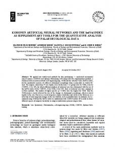
Figure 1a shows an example of using the new EKF learning algorithm for feed-forward neural networks for the CH4 -N2 O correlation from the Cambridge 2D model (Law and Pyle, 1993a,b) (red crosses with validation points as green crosses). The CH4 -N2 O data is shown by the yellow filled blue circles. The correlation coefficient between the actual solution and the neural network solution was 0.9997 after just 200 iterations (epochs). The same correlation coefficient is obtained after just 3 iterations (epochs). Overlaid on the same panel are the previous results of Lary et al. (2004) (cyan crosses) 6 which used “Quickprop” learning and required 10 iterations to reproduce the CH4 N2 O correlation with a correlation coefficient between simulated and training values of 0.9995. So the new algorithm gives better results with much less expense. Figure 1b 3660
Abstract
Introduction
Conclusions
References
Tables
Figures
J
I
J
I
Back
Close
Full Screen / Esc
Print Version Interactive Discussion
© EGU 2004
5
10
15
shows a scatter diagram of the known N2 O concentration against the neural network N2 O concentration. Figure 1c shows the way the rms error changes with epoch. Both CH4 and pressure are strongly correlated with N2 O as can be seen in Fig. 1 of Lary et al. (2004). Latitude and time are only weakly correlated with N2 O but still play a small role in capturing some of the details of the CH4 -N2 O correlation in Panel (a). A polynomial or other fit will typically do a good job of describing the CH4 -N2 O correlation for high values of CH4 and N2 O. However, for low values of CH4 and N2 O there is quite a spread in the relationship which a single curve can not describe. This is the altitude dependent regime where the correlation shows significant variation with altitude (Minschwaner et al., 1996). Figure 1a shows a more conventional fit using a Chebyshev polynomial of order 20 overlaid on the neural network fits. This fit was chosen as giving the best agreement to the CH4 -N2 O correlation after performing fits using 3667 different equations. Even though this is a good fit the spread of values can not be described by a single curve. However, a neural network trained with the latitude, pressure, time of year, and CH4 volume mixing ratio (v.m.r.) (four inputs) is able to well reproduce the N2 O v.m.r. (one output), including the spread for low values of CH4 and N2 O. 3.1. Scaling
20
Variable scaling often allows neural networks to achieve better results. In this case all variables were scaled to vary between ±1. If the initial range of values was more than an order of magnitude then log scaling was also applied. In the case of time of year the sine of the fractional time of year was used to avoid a step discontinuity at the start of the year.
ACPD 4, 3653–3667, 2004
Neural networks and tracer correlations D. J. Lary and H. Y. Mussa
Title Page Abstract
Introduction
Conclusions
References
Tables
Figures
J
I
J
I
Back
Close
Full Screen / Esc
Print Version Interactive Discussion
© EGU 2004 3661
4. Conclusions
5
10
15
20
25
ACPD
Neural networks are ideally suited to describe the spatial and temporal dependence of tracer-tracer correlations. Even in regions when the correlations are less compact. Using a new extended Kalman filter learning algorithm for feed-forward neural networks the correlation coefficient between the actual solution and the neural network solution was 0.9997 after just 200 iterations (epochs). The same correlation coefficient is obtained after just 3 iterations (epochs). This can be compared to our previous study (Lary et al., 2004) which used “Quickprop” learning and required 106 iterations to reproduce the CH4 -N2 O correlation with a correlation coefficient between simulated and training values of 0.9995. So the new algorithm gives better results with much less expense. Acknowledgements. It is a pleasure to acknowledge: NASA for a distinguished Goddard Fellowship in Earth Science; The Royal Society for a Royal Society University Research Fellowship; The government of Israel for an Alon Fellowship; The NERC, EU, and ESA for research support.
4, 3653–3667, 2004
Neural networks and tracer correlations D. J. Lary and H. Y. Mussa
Title Page Abstract
Introduction
Conclusions
References
Tables
Figures
References
J
I
Bierman, G.: Factorization Methods for Discrete Sequential Estimation, Academic Press, 1977. 3655, 3656, 3660 Bishop, C.: Neural Networks for Pattern Recognition, Oxford University Press, 1996. 3655 Blank, T. B. and Brown, S. D.: Adaptive, global, extended Kalman filters for training feedforward neural networks, Journal of Chemometrics, 8, 391–407, 1994. 3655 Elkins, J. W., Fahey, D. W., Gilligan, J. M., Dutton, G. S., Baring, T. J., Volk, C. M., Dunn, R. E., Myers, R. C., Montzka, S. A., Wamsley, P. R., Hayden, A. H., Butler, J. H., Thompson, T. M., Swanson, T. H., Dlugokencky, E. J., Novelli, P. C., Hurst, D. F., Lobert, J. M., Ciciora, S. J., McLaughlin, R. J., Thompson, T. L., Winkler, R. H., Fraser, P. J., Steele, L. P., and Lucarelli, M. P.: Airborne gas chromatograph for in situ measurements of long-lived species in the upper troposphere and lower stratosphere, Geophys. Res. Lett., 23, 347–350, 1996. 3654
J
I
Back
Close
3662
Full Screen / Esc
Print Version Interactive Discussion
© EGU 2004
5
10
15
20
25
30
Fahey, D. W., Murphy, D. M., Kelly, K. K., Ko, M. K. W., Proffitt, M. H., Eubank, C. S., Ferry, G. V., Loewenstein, M., and Chan, K. R.: Measurements of nitric-oxide and total reactive nitrogen in the antarctic stratosphere – observations and chemical implications, J. Geophys. Res. (Atmos.), 94, 16 665–16 681, 1989. 3654 Fischer, H., Wienhold, F. G., Hoor, P., Bujok, O., Schiller, C., Siegmund, P., Ambaum, M., Scheeren, H. A., and Lelieveld, J.: Tracer correlations in the northern high latitude lowermost stratosphere: Influence of cross-tropopause mass exchange, Geophys. Res. Lett., 27, 97– 100, 2000. 3654 Haykin, S.: Kalman Filtering and Neural Networks, Wiley-Interscience, 2001. 3657, 3658, 3659 Iiguni, Y., Sakai, H., and Tokumaru, H.: A real-time learning algorithm for a multilayered neural network based on the extended Kalman filter, IEEE Transactions on Signal Processing, 40, 959–966, 1992. 3655 Keim, E. R., Loewenstein, M., Podolske, J. R., Fahey, D. W., Gao, R. S., Woodbridge, E. L., Wamsley, R. C., Donnelly, S. G., DelNegro, L. A., Nevison, C. D., Solomon, S., Rosenlof, K. H., Scott, C. J., Ko, M. K. W., Weisenstein, D., and Chan, K. R.: Measurements of the NOy -N2 O correlation in the lower stratosphere: Latitudinal and seasonal changes and model comparisons, J. Geophys. Res. (Atmos.), 102, 13 193–13 212, 1997. 3654 Lary, D. J., Muller, M. D., and Mussa, H. Y.: Using neural networks to describe tracer correlations, Atmospheric Chemistry and Physics, 4, 143–146, 2004. 3655, 3660, 3661, 3662, 3667 Law, K. and Pyle, J.: Modeling trace gas budgets in the troposphere .1. O3 and odd nitrogen, J. Geophys. Res. (Atmos.), 98, 18 377–18 400, 1993a. 3660 Law, K. and Pyle, J.: Modeling trace gas budgets in the troposphere .2. CH4 and CO, J. Geophys. Res. (Atmos.), 98, 18 401–18 412, 1993b. 3660 Loewenstein, M., Podolske, J. R., Fahey, D. W., Woodbridge, E. L., Tin, P., Weaver, A., Newman, P. A., Strahan, S. E., Kawa, S. R., Schoeberl, M. R., and Lait, L. R.: New observations of the NOy /N2 O correlation in the lower stratosphere, Geophys. Res. Lett., 20, 2531–2534, 1993. 3654 Lonnblad, L., Peterson, C., and Rognvaldsson, T.: Pattern-recognition in high-energy physics with artificial neural networks – “JETNET-2.0”, Comp. Phys. Comm., 70, 167–182, 1992. 3655 Michelson, H. A., Manney, G. L., Gunson, M. R., and Zander, R.: Correlations of stratospheric
3663
ACPD 4, 3653–3667, 2004
Neural networks and tracer correlations D. J. Lary and H. Y. Mussa
Title Page Abstract
Introduction
Conclusions
References
Tables
Figures
J
I
J
I
Back
Close
Full Screen / Esc
Print Version Interactive Discussion
© EGU 2004
5
10
15
20
25
30
abundances of NOy , O3 , N2 O, and CH4 derived from ATMOS measurements, J. Geophys. Res. (Atmos.), 103, 28 347–28 359, 1998. 3654 Minschwaner, K., Dessler, A. E., Elkins, J. W., Volk, C. M., Fahey, D. W., Loewenstein, M., Podolske, J. R., Roche, A. E., and Chan, K. R.: Bulk properties of isentropic mixing into the tropics in the lower stratosphere, J. Geophys. Res. (Atmos.), 101, 9433–9439, 1996. 3661 Morgenstern, O., Lee, A. M., and Pyle, J. A., Cumulative mixing inferred from stratospheric tracer relationships, J. Geophys. Res. (Atmos.), 108, 2002. 3654 Muscari, G., de Zafra, R. L., and Smyshlyaev, S.: Evolution of the NOy -N2 O correlation in the antarctic stratosphere during 1993 and 1995, J. Geophys. Res. (Atmos.), 108, 2003. 3654 Peterson, C., Rognvaldsson, T., and Lonnblad, L.: “JETNET 3.0” a versatile artificial neural network package, Comp. Phys. Comm., 81, 185–220, 1994. 3655 Plumb, R. A. and Ko, M. K. W.: Interrelationships between mixing ratios of long lived stratospheric constituents, J. Geophys. Res. (Atmos.), 97, 10 145–10 156, 1992. 3654 Puskorius, G. V. and Feldkamp, L. A.: Neurocontrol of nonlinear dynamical-systems with kalman filter trained recurrent networks, IEEE Transactions on Neural Networks, 5, 279– 297, 1994. 3656 Rinsland, C. P., Salawitch, R. J., Gunson, M. R., Solomon, S., Zander, R., Mahieu, E., Goldman, A., Newchurch, M. J., Irion, F. W., and Chang, A. Y.: Polar stratospheric descent of NOy and CO and arctic denitrification during winter 1992-1993, J. Geophys. Res. (Atmos.), 104, 1847–1861, 1999. 3654 Schoeberl, M. R., Roche, A. E., Russell, J. M., Ortland, D., Hays, P. B., and Waters, J. W.: An estimation of the dynamical isolation of the tropical lower stratosphere using UARS wind and trace gas observations of the quasibiennial oscillation, Geophys. Res. Lett., 24, 53–56, 1997. 3654 Shah, S., Palmieri, F., and Datum, M.: Optimal filtering algorithms for fast learning in feedforward neural networks, Neural Networks, 5, 779–787, 1992. 3655, 3656, 3657 Singhal, S. and Wu, L.: Training feedforward networks with extended Kalman filter algorithm, in Proc. Int. Conf. ASSP, pp. 1187–1190, 1989. 3655, 3656 Strahan, S. E., Climatologies of lower stratospheric NOy and O3 and correlations with N2 O based on in situ observations, J. Geophys. Res. (Atmos.), 104, 30 463–30 480, 1999. 3654 Watrous, R.: Learning algorithms for connectionist networks, in Proc. IEEE First Int. Conf. Neural Networks, 2, p. 619, 1987. 3655 Waugh, D. W. and Funatsu, B. M.: Intrusions into the tropical upper troposphere: Three-
3664
ACPD 4, 3653–3667, 2004
Neural networks and tracer correlations D. J. Lary and H. Y. Mussa
Title Page Abstract
Introduction
Conclusions
References
Tables
Figures
J
I
J
I
Back
Close
Full Screen / Esc
Print Version Interactive Discussion
© EGU 2004
285
dimensional structure and accompanying ozone and olr distributions, J. Atmos. Sci., 60, 637–653, 2003. 3654 Zhang, Y. M. and Li, X. R.: A fast u-d factorization-based learning algorithm with applications to nonlinear system modeling and identification, IEEE Transactions on Neural Networks, 10, 930–938, 1999. 3656, 3657, 3659, 3660
ACPD 4, 3653–3667, 2004
Neural networks and tracer correlations D. J. Lary and H. Y. Mussa
Title Page Abstract
Introduction
Conclusions
References
Tables
Figures
J
I
J
I
Back
Close
Full Screen / Esc
Print Version Interactive Discussion
© EGU 2004 3665
Lary: Neural Networks and Tracer Correlations
ACPD
3
4, 3653–3667, 2004
CH4−N2O
Neural networks and tracer correlations
−7
10
2
N O
D. J. Lary and H. Y. Mussa −8
10
Title Page Known N O vs CH 2 4 Lary et al. (2004) N O vs CH 2 4 Predicted N O vs CH 2 4 Validation N O vs CH
−9
2
10
4
Abstract
Introduction
Conclusions
References
Tables
Figures
J
I
J
I
Back
Close
Chebyshev Polynomial Order 20 0.5
1
1.5
2
2.5
CH4
(a) Scatter plot of Known vs Predicted N2O
−6
x 10
RMS error vs Epochs 0.09 0.08
−7
10
RMS error
Known N2O
0.07
−8
10
0.06 0.05
Full Screen / Esc
0.04 0.03
−9
−9
10
(b)
−8
10
NN N2O
Print Version
0.02
Correlation coefficient 0.9997
10
0.01 0 10
−7
10
(c)
1
10
2
10
Fig. 1. The neural network used to produce the CH4 -N2 O correlation in Panel (a) is our new extended Kalman filter learning algorithm for feed-forward neural networks (red crosses with validation points as green crosses). The data is shown by the yellow filled blue circles. The correlation coefficient between the actual solution and the neural network solution was 0.9997 after just 200 iterations (epochs). The same correlation coefficient is obtained after just 3 iterations (epochs). Overlaid on the same panel are the previous results of Lary et al. (2004) (cyan crosses) which used Quickprop learning and required 106 iterations to reproduce the CH4 -N2 O correlation with a correlation coefficient between simulated and training values of 0.9995. A Chebyshev polynomial of order 20 is also shown (small black circles) for the sake of comparison. This fit was chosen as giving the best agreement to the CH4 -N2 O correlation after performing fits using 3667 different
3666
Interactive Discussion
Number of Epochs
© EGU 2004
ACPD 4, 3653–3667, 2004
Neural networks and tracer correlations
Fig. 1. The neural network used to produce the CH4 -N2 O correlation in (a) is our new extended Kalman filter learning algorithm for feed-forward neural networks (red crosses with validation points as green crosses). The data is shown by the yellow filled blue circles. The correlation coefficient between the actual solution and the neural network solution was 0.9997 after just 200 iterations (epochs). The same correlation coefficient is obtained after just 3 iterations (epochs). Overlaid on the same panel are the previous results of Lary et al. (2004) (cyan crosses) which 6 used “Quickprop” learning and required 10 iterations to reproduce the CH4 -N2 O correlation with a correlation coefficient between simulated and training values of 0.9995. A Chebyshev polynomial of order 20 is also shown (small black circles) for the sake of comparison. This fit was chosen as giving the best agreement to the CH4 -N2 O correlation after performing fits using 3667 different equations. Even though this is a good fit the spread of values can not be described by a single curve. However, a neural network trained with the latitude, pressure, time of year, and CH4 volume mixing ratio (v.m.r.) (four inputs) is able to well reproduce the N2 O v.m.r. (one output), including the spread for low values of CH4 and N2 O. (b) shows a scatter diagram of the known N2 O concentration against the neural network N2 O concentration. (c) shows the way the rms error changes with epoch.
D. J. Lary and H. Y. Mussa
Title Page Abstract
Introduction
Conclusions
References
Tables
Figures
J
I
J
I
Back
Close
Full Screen / Esc
Print Version Interactive Discussion
© EGU 2004 3667