Control and Cybernetics vol.
39 (2010) No. 1
Neural networks as performance improvement models in intelligent CAPP systems∗ by Izabela Rojek Kazimierz Wielki University in Bydgoszcz Institute of Mechanics and Applied Computer Science Bydgoszcz, Poland e-mail:
[email protected] Abstract: The paper presents neural networks as performance improvement models in intelligent computer aided process planning systems (CAPP systems). For construction of these models three types of neural networks were used: linear network, multi-layer network with error backpropagation, and the Radial Basis Function network (RBF). The models were compared. Due to the comparison, we can say which type of neural network is the best for selection of tools for manufacturing operations. Tool selection for manufacturing operation is a classification problem. Hence, neural networks were built as classification models, meant to improve tool selection for manufacturing. The study was done for selected manufacturing operations: turning, milling and grinding. Models for the milling operation were presented in detail. Keywords: classification model, neural network, tool, manufacturing operation.
1.
Introduction
Nowadays, knowledge is treated as the basic and most valuable enterprise resource and a factor of enterprise development. It is a specific type of resource in contrast to the other ones it grows with its use. Currently the most difficult problem in the creation of systems of knowledge acquisition is to obtain knowledge and experience from enterprise employees, as they are reluctant to share their knowledge with others. That is why data mining is so important (Hand, Mannila and Smith, 2005; Larose, 2006; Michalski, Bratko and Kubat, 1998; and Monostori et al., 1996). Data mining involves processes that cannot be automated, but must be operated by a user. There are six basic steps which render the data mining process effective: ∗ Submitted:
February 2009; Accepted: July 2009.
56
I. ROJEK
1. Understanding and properly defining the problem/task which is the object of mining. Moreover, the background or surroundings, in which the problem occurs, should also be properly examined. 2. Selecting the set of data to be subject to mining. The set has to be a substantial sample of the entire data on the problem. The selection refers to objects, their attributes (variables), span of time, geographical area, the size of sample etc. 3. Deciding how to prepare data for processing. For example: should age be represented as a range (for example 40-45 years) or as a definite figure (for example 40 years). 4. Selecting algorithm(s) of data mining and writing respective code for the prepared data. Very often there is a need to go back to step 3 or even 2 if the results are unsatisfactory. 5. Analyzing the results of code execution and choosing the ones, which constitute the proper output from the work. At this stage, close cooperation between an analyst and a specialist in the explored area is needed. The results should be presented in the commonly accepted form in the organization in question. 6. Submitting the results to the management of the organization and suggesting their possible application. Data mining techniques - decision trees, neural networks, and regression are implemented as different tools. Data mining focuses on making clients aware of the complexity of data they have at their disposal and the possibilities of using these data effectively. For purposes of data mining, data warehouses collecting data from different, also global sources, are constructed. The need to develop models that use neural nets in intelligent support results from the defects of the methods previously applied to solve this type of problems: database application or traditional expert systems (Weiss and RojekMikołajczak, 1993, 1997; Rojek-Mikołajczak and Weiss, 1999; Rojek, 2005). In database applications, the relational model was too poor a model of data. Two dimensionality of the relational database causes the flattening of multidimensional data model related to the manufacturing process. The database contains only data (facts), not knowledge, or the reasoning mechanism, or the ability of acquiring knowledge in reasoning process, or autolearning (see Banachowski, 1998, and Beynon-Davies, 2000). Traditional expert systems have difficulty in knowledge acquisition and checking the correctness of the knowledge base. The cost and time of expert system design grow with the increase of the number of rules, and the large number of rules causes problems with the management of reasoning processes (Bubnicki, 1990; Mulawka, 1996). The article presents the practical aspect of the problem of intelligent selection of tools for manufacturing operation. This is a classification problem. Therefore, neural networks, used here, were built as models of classification.
Neural networks as performance improvement models in intelligent CAPP systems
57
The paper presents and compares classification models in the form of selected types of neural networks: multi-layer network with error backpropagation, linear network, and the network with radial basic functions. Due to comparison, we can indicate the type of neural network that is the best for selection of tools for manufacturing operations. The models improve the performance of tool selection for manufacturing operation. These models are a new approach to solving the problem of selection of tools.
2.
Neural network as a classification model
Neural networks return continuous value at the output, hence they are excellent for estimating and classifying. Such networks may analyze many variables at a time. It is possible to create a model, even if solution is very complex. The drawbacks of neural networks are the difficulty in setting architectural parameters, falling into local minima, long learning process and lack of clear interpretation (Krawiec and Stefanowski, 2004; Rutkowska, Piliński and Rutkowski, 1997; Rutkowski, 2005, and Tadeusiewicz, 1993). Three types of neural networks were used for construction of the classification model. In multi-layer network with error backpropagation, the signals flow from input to output. Multi-layer networks are formed with many layers of neurons. The input of each neuron from a given layer is linked with outputs of all neurons in the preceding layer. The first layer is called the input layer, the last output layer, and the rest are hidden layers. The number of layers and neurons is random. Identification of the model structure answers the following questions: • How many layers does the neural network consist of (are hidden layers required)? • How many neurons does each layer contain? • Is it necessary to include an extra neuron to ensure a better network stability during the learning process (bias)? How to refine learning parameters of the network (learning rate, momentum factor etc.)? Identification of the parameters of the model consists in the refinement of the interneuron connection weights. Connection weights are being adjusted until the root mean square variable reaches minimum, which allows for the termination of the learning process. The number of hidden layers and the number of neurons in these layers greatly influence the operational quality of a layered network. Most often, the number of hidden neurons is determined on experimental basis. The problem here is quite complicated: too few hidden neurons prevent the network from acquiring sufficient knowledge on the problem solved; whereas an overly complex architecture results in the so-called generalization "handicap" (the network renders the training set too precisely, creating generalization problems with regard to cases not included in the learning process).
58
I. ROJEK
The above predicament is usually solved through experimental means. Multiple recurrences of the learning process allow for designing networks which are large enough to "learn" the given problem, and at the same time small enough to generalize correctly. Verification of the neural network model consists in testing, verification and adjustment. Testing examines network operation on data included in a test file. Verification allows for ensuring that the network selects correct output parameters for new input variables. Adjustment consists of a change in the number of neurons in the network, extension of the learning process if the network is over-trained or a change in the number of hidden layers. In order to assess the quality of knowledge acquired by the network during learning, three factors have been used: Root-Mean-Square Error (RMS), learning (training) tolerance and testing tolerance. The user can trace the above factors, and as a result determine the moment of termination of the learning process. RMS Error is the standard error given by the formula of the sum of squared deviations of the actual and desired values, divided subsequently by the number of these values. The drawback of this standard lies in the fact that it does not reflect an error of a single network output. However, it allows for the definition of the mean deviation in the training set presentation cycle. Therefore, a tolerance factor is checked as well, defining an acceptable error of a single network output. Tolerance factor correlates with sets outside tolerance, and shows the number of sets included in a group outside the current tolerance variable for the network outputs. The here applied neuron model is of sigmoid type (Duch, 2000). It consists of the sum element joined by input signals x1 , x2 , ..., xN in the form of an input vector x = [x1 , x2 , ..., xN ]T multiplied by weights wi1 , wi2 , ..., wiN in the form of a weight vector of ith neuron wi = [wi1 , wi2 , ..., wiN ]T and the value wi0 . The signal of the sum element is marked ui : X ui = wij xj + wi0 (1) and the signal is given to a non-linear activation function f (ui), being a unipolar sigmoid function: fu (ui ) =
1 . 1 + exp (−βui )
(2)
Linear network is a network with no hidden layers, and the neurons in the output layer are fully linear (i.e. these are neurons, whose collective stimulation is determined as a linear combination of input values and which have a linear activation function). During the operation of the network, the inputs are multiplied by a weight matrix, which collectively forms a vector of output signals. RBF - Radial Basis Function network usually has one hidden layer with radial neurons, each of which models a Gaussian surface of responses. Since
Neural networks as performance improvement models in intelligent CAPP systems
59
these functions are strongly non-linear, one hidden layer is enough to model a function of any shape. Yet, for an RBF to form a successful model of any function, the network structure needs to dispose of many radial neurons. If there is a sufficient number of radial neurons, each important detail of a modeled function can have the needed radial neuron attached, which guarantees that the obtained solution shall genuinely reproduce the given function. Radial networks consist of neurons, whose activation functions are x 7→ ϕ(kx − ck), x ∈ Rn
(3)
where (k·k) is the Euclidean norm. Functions ϕ(kx − ck) are called radial base functions. Their values change radially from the centre c. A radial neuron is defined by its centre and a parameter defined as "ray". Neurons in the hidden layer are defined by formula (3). A neuron in output layer stands for the operation of the weighed sum of signals of output neurons in the hidden layer, and can be expressed as X X wi ϕ(kx − ci k). (4) wi ϕi = y= i
3.
i
The method of development of performance improvement models
The method developed allows for creating the models according to the algorithm of Fig. 1. The algorithm consists of the following steps: 1. Mark the model type: classification, prediction, preference. 2. Mark the artificial intelligence method: neural network, decision tree, multiple decision trees. 3. Determine the learning and testing set. 4. Create the model from scratch: • Determine the initial parameters of the model. • Determine the structure of the model. • Carry out the procedure of model learning. • Stop criterion satisfied (RMS = RMSmin)?; stop criteria other than RMS can be used, if ’Yes’, move to testing procedure. • Carry out the procedure of model testing. • Stop criterion satisfied (RMS = RMSmin)?, stop criteria other than RMS can be used, if ’Yes’, show the parameters of the model. • Introduce the model to model base. • Do you want to create a new model? If ’Yes’, go to the stage of updated learning of the model. If ‘No’ then STOP.
60
I. ROJEK
Figure 1. Algorithm of model base development
Neural networks as performance improvement models in intelligent CAPP systems
61
5. In the case of updated learning of the model on new data: • Choose the model for update learning. • Carry out the procedure of model learning. • Stop criterion satisfied (RMS = RMSmin)?; stop criteria other than RMS can be used, if ’Yes’, move to testing procedure. • Carry out the procedure of model testing. • Stop criterion satisfied (RMS = RMSmin)?; stop criteria other than RMS can be used, if ’Yes’, show the parameters of the model. • Introduce the model to model base. • Do you want to create a new model? If ’Yes’, go back to the stage of updated learning of the model. If ’No’ then STOP.
4.
Neural model for selection of tools for manufacturing operations
Experiments were carried out for selected manufacturing operations: turning, milling and grinding. For each operation, three models were drawn using three types of neural networks: linear network, multi-layer network with error backpropagation and RBF network. For each type of network, a comparison as to which network produced best results was done. The paper is illustrated with selected models. The aim of the task was selection of a tool for manufacturing operation on the basis of given input parameters (Chlebus, 2000; Feld, 2000; and Weiss, 1998). Evaluation gain was the effectiveness of tool selection with a certain group of tools possible to select. The bigger the number of tools correctly classified, the better. Experience was represented by database gathered in an enterprise. We suppose that a representative number of tool selection cases is located in database. Representation of learning cases occurs most often in attributevalue notation. Therefore, we suppose that the file of learning examples is described by means of established attribute file, which possesses certain features characterizing properties of objects described in the file of examples. In practice, the examples are represented in table form with rows corresponding to examples, and columns to attributes. Additionally, aside from the file of learning examples the file of test examples can be created. The format of both files is the same. 4.1.
Data preparation
Correctness of acquired knowledge greatly depends on examples, on the basis of which the methods of knowledge acquisition work. Initial data processing plays an important role during learning and testing of neural networks. At this stage, we must solve such problems as proper selection of features or right examples.
62
I. ROJEK
Certain additional problems limiting the choice of optimal feature set, such as the problem of dimensionality, data correlation, or data interrelationship, combine with the right selection of features. Learning and testing files were prepared with the aim of knowledge acquisition aiding tool selection for manufacturing operation, separately for turning, milling and grinding. Learning files include about 900 examples, whereas testing files about 200. Input attributes are nominal, ordinal and numeric type. The files are decision tables, in which the last column in table is a decision attribute (tool symbol). "Data purification" process was carried out. An accurate data profiling, data parsing, data verification (on the levels of field, row and table) and data standardization was carried out. Duplicates were removed, as well. The examples included in the files are real tool selections performed during design of manufacturing processes in an enterprise. In the case of turning, input data include: • the kind of turning (e.g. roughing), • turning cut (e.g. straight), • stock symbol (e.g. St3W), • type of stock (e.g. soft), • turning tool structure (e.g. monolithic), • kind of turning tool (e.g. left-cut tool). Output datum is turning tool symbol (e.g. 23600). In the case of milling, input data include (Rojek, 2007): • the kind of milling (e.g. roughing), • type of machining surface (e.g. surface), • stock symbol (e.g. 1,053), • demanded surface roughness (e.g. 40), • milling tool structure (e.g. inserted-tooth cutter), • the kind of milling tool clamping (e.g. arbor), • dimension (e.g. 160), • tooth number (e.g. 10), • total length of milling tool (e.g. 300). Output datum is the milling tool symbol (e.g. hR 257.1-160) (Fig. 2).
Figure 2. A fragment of the learning file
63
Neural networks as performance improvement models in intelligent CAPP systems
In the case of grinding, input data include: • the kind of grinding (e.g. roughing), • grinding cut (e.g. surface), • stock symbol (e.g. 1,053), • demanded surface roughness (e.g. 40), • external dimension of grinding wheel (e.g. 80), • internal dimension of grinding wheel (e.g. 30), • grain size (e.g. 540), • structure of grinding wheel (e.g. compact). Output datum is grinding wheel symbol (e.g. 56350). 4.2.
Neural network models for classification
The models were created according to the algorithm from Fig. 1. Model of a multi-layer neural network with error backpropagation The model of a multi-layer neural network with error backpropagation (MLP) is equipped with eleven inputs, one output and one hidden layer containing 5, 10 or 15 neurons. In the hidden layer of the network, the number of neurons was selected experimentally. Network inputs include manufacturing conditions of tool selection. Network output constitutes a set of values determining results received during tool selection for given conditions. These structures were learnt with different conditions of ending the process, i.e. after reaching the number of periods equal to 1 000, 10 000 or 100 000. For every combination, classification error was established, based on entropy function. Fig. 3 illustrates the parameters of different structures of MLP networks. Type of network Learning Testing structure quality quality
Learning Testing error error
Number of inputs
Number of hidden layer neurons
MLP 11-5-1
0.914414 0.905405
0.378654 0.451943
11
5
MLP 11-10-1
0.975225 0.977477
0.230815 0.237306
11
10
MLP 11-15-1
0.959459 0.900901
0.234178 0.503807
11
15
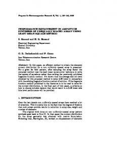
Figure 3. Parameters of MLP networks Hence, the neural network MLP-11-10-1 proved to be the most accurate model when the learning process was stopped after 1 000 periods. Results obtained for the new input values proved the point. Fig. 4 illustrates the ratios of proper classification for different milling cutters and different structures of MLP neural networks (Rojek, 2008).
64
I. ROJEK
5 neurons
10 neurons
15 neurons
120,00 100,00 80,00 60,00 40,00 20,00 mill_symbol.20507.1
mill_symbol.20400.1
mill_symbol.20511.1
mill_symbol.20355.1
mill_symbol.20505.1
mill_symbol.20402.1
mill_symbol.NFPc.1
mill_symbol.NFPa.1
mill_symbol.CMD12-A-W12.1
mill_symbol.220.17100.1
mill_symbol.220.1780.1
mill_symbol.220.1750.1
mill_symbol.220.1763.1
mill_symbol.F90APD40-22.1
mill_symbol.NFMa.1
mill_symbol.hR 257.1-160.1
mill_symbol.hR 257.1-200.1
mill_symbol.NFPg.1
mill_symbol.20340.1
0,00
Figure 4. Analysis of proportions of proper classification for different milling cutters Averages of proper classification of milling cutters from Fig. 4 are as follows: • 88.16 % for the structure with 5 neurons in hidden layer, • 97.59 % for the structure with 10 neurons in hidden layer, • 94.02 % for structure with 15 neurons in hidden layer. The averages were calculated for classification of all milling cutters used in the experiment.
Linear network model Similar experiment was done for the linear network model. Yet, in this case, only a model with eleven inputs and one output was tried out. This structure was learnt, as before, for 1 000, 10 000 or 100 000 periods. Classification error was calculated for every combination. The neural network obtained after 1000 periods had the following parameters: • learning quality (0.743243), • testing quality (0.725225), • learning error (0.162979), • testing error (0.164048). Average ratio of proper classification of milling cutters, based on Fig. 7 is 54.37%.
65
Neural networks as performance improvement models in intelligent CAPP systems
RBF network model The model of an RBF neural network was drawn was equipped with eleven inputs and one output and one hidden layer containing 10, 15, 20 or 25 neurons. As before, learning was stopped after 1 000, 10 000, or 100 000 periods. For every combination, classification error was established. Fig. 5 shows parameters of different structures of RBF networks. Type of network Learning Testing structure quality quality
Learning Testing error error
Number of inputs
Number of Hidden Layer Neurons
RBF 11-10-1
0.421171 0.396396
2.046189 2.151990
11
10
RBF 11-15-1
0.527027 0.454955
1.354457 1.448193
11
15
RBF 11-20-1
0.695946 0.621622
1.179801 1.332639
11
20
RBF 11-25-1
0.662162 0.599099
1.279110 1.378898
11
25
Figure 5. Parameters of RBF networks It can be seen from Fig. 5 that neural network RBF 11-20-1 proved to be the most accurate model. The results obtained for the new input values proved the point. The average ratio of proper classification of milling cutters (see Fig. 7) is 51.19%. The models of RBF networks learned on a small learning file have too big learning and testing errors (Fig. 5). Hence, we changed the learning file, and RBF networks were subject to update learning. Comparison of classification models All these models classify tools for manufacturing operations. The models were tested on selected manufacturing operations. MLP model proved to be the most accurate. Fig. 6 shows those parameters the MLP, Linear and RBF networks selected, under comparable conditions (the same termination conditions). Type of network Learning Testing structure quality quality
Learning Testing error error
Number of inputs
Number of hidden layer neurons
MLP 11-10-1
0.975225 0.977477
0.230815 0.237306
11
Linear 11-1
0.743243 0.725225
0.162979 0.164048
11
10 0
RBF 11-20-1
0.695946 0.621622
1.179801 1.332639
11
20
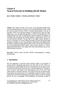
Figure 6. Parameters of the best MLP, Linear and RBF networks Fig. 7 presents graphically the comparison between the proportions of proper classification of tools for milling operations for the neural networks used in the experiment. Updated learning of the neural networks on the basis of additional examples of tools selection, showed the improvement in the RBF network performance.
66
I. ROJEK
mill_symbol.20507.1
mill_symbol.20400.1
mill_symbol.20511.1
mill_symbol.20355.1
mill_symbol.20505.1
mill_symbol.20402.1
mill_symbol.NFPc.1
mill_symbol.CM-
RBF
mill_symbol.NFPa.1
mill_symbol.220.17-
Linear
mill_symbol.220.17-
mill_symbol.220.17-
mill_symbol.F90AP-
mill_symbol.220.17-
mill_symbol.NFMa.1
mill_symbol.hR
mill_symbol.hR
mill_symbol.NFPg.1
120,00 100,00 80,00 60,00 40,00 20,00 0,00
mill_symbol.20340.1
MLP
Figure 7. Comparison of classification models The updated RBF network correctly classified the tools in 98%. The parameters of this RBF network are: learning quality - 0.985032, testing quality – 0.982345, learning error – 0.191798, and testing error – 0.194363. Using neural networks as classification models, application meant to aid a process engineer in selecting tools for manufacturing operation was implemented. This tool selection application works in a dialogue mode, and queries the process engineer about input attributes and gives answers in the form of tool symbols.
5.
Summary
The general principle of science states that if there is a possibility to choose between a complex and a simple model, the simple model should always be given priority – unless, of course, the more complex one is significantly better than the simple one for the particular problem. This principle should also be applied to neural networks. Having analyzed various classification models for milling, we found that the MLP network model proved most effective. Moreover, experiments were performed concerning tool selection for other manufacturing operations: grinding and turning. The MLP neural networks were the best models in case of these other operations, too. Network model was tested on data from testing file and network activity was tested for new input values.
Neural networks as performance improvement models in intelligent CAPP systems
67
However, updated learning of the neural networks on the basis of additional examples of tool selection, showed a significant improvement in the RBF network performance. RBF network correctly classified tools in 98%. Using neural networks as classification models, application having aid process engineer in selection of tools for manufacturing operation was implemented. The system here described, enables the acquisition of data, knowledge and experience of a process engineer in its entirety. With a view to meeting the aim of the research, the existing databases of an enterprise were used, along with the decision rules of expert system and neural network models. The comprehensive method of knowledge acquisition is a considerable achievement when compared to traditional expert systems based on human expert-derived knowledge. The advantage of the method is substantial, especially when such knowledge is inaccessible, difficult to formalize or unreliable. When acquiring new data, these models should be learnt in any moment in time. Further research into when and how to learn these models should be done. The traditional computer systems only support the design of the manufacturing process. However, application of the neural networks significantly improves the performance of the intelligent CAPP systems.
References Banachowski, L. (1998) Bazy danych. Tworzenie aplikacji (Databases. Developing the applications; in Polish). Akademicka Oficyna Wydawnicza PLJ, Warszawa. Beynon-Davies, P. (2000) Systemy baz danych (Database Systems; Polish translation). WNT, Warszawa. Bubnicki, Z. (1990) Wstęp do systemów ekspertowych (An Introduction to expert systems; in Polish). PWN, Warszawa. Chlebus, E. (2000) Techniki CAx w inżynierii produkcji (CAx Computer Techniques in Production Engineering; in Polish). WNT, Warszawa. Duch, W., Korbicz, J., Rutkowski, L. and Tadeusiewicz, R. (2000) Sieci neuronowe, Biocybernetyka i Inżynieria Biomedyczna (Neural Networks, Biocybernetics and Biomedical Engineering; in Polish), 6. Academic Publishing House EXIT, Warszawa. Feld, M. (2000) Podstawy projektowania procesów technologicznych typowych części maszyn (Elements of Manufacturing Processes Design of Typical Machine Parts; Polish translation). WNT, Warszawa. Hand, D., Mannila, H. and Smith, P. (2005) Eksploracja danych (Principles of Data Miting; Polish translation). WNT, Warszawa. Krawiec, K. and Stefanowski, J. (2004) Uczenie maszynowe i sieci neuronowe (Machine Learning and Neural Networks; in Polish). Publishing House of Poznan University of Technology, Poznań. Larose, D. T. (2006) Odkrywanie wiedzy z danych. Wprowadzenie do eksploracji danych (Discovering Knowledge in Data. An Introduction to Data
68
I. ROJEK
Mining). PWN. Warszawa (in Polish) Michalski, R.S., Bratko, I. and Kubat, M. (1998) Machine Learning and Data Mining. John Wiley&Sons, New York. Monostori, L., Markus, A., Brussel, H.V. and Westkämpfer, E. (1996) Machine learning approaches to manufacturing. Annals of the CIRP, 45 (2), 675-712. Mulawka, J. (1996) Systemy ekspertowe (Expert Systems; in Polish). WNT, Warszawa. Rojek-Mikołajczak, I. and Weiss, Z. (1999) Intelligent databases for CAPP. Proceedings of the 10th Int. DAAAM Symposium, Vienna, 471-472. Rojek, I. (2005) Bazy danych i bazy wiedzy w zarządzaniu wiedzą technologiczną przedsiębiorstwa (Databases and knowledge bases for manufacturing knowledge management of enterprise). In: S. Kozielski et al., eds., Bazy Danych – Modele, Technologie, Narzędzia (Databases - Models, Technologies, Tools; in Polish). Wydawnictwo Komunikacji i Łączności, Warszawa, 257-264. Rojek, I. (2007) Knowledge Discovery for Computer Aided Process Planning Systems. Polish Journal of Environmental Studies 16 (4A), 268-270. Rojek, I. (2008) Neural networks as classification models in intelligent CAPP systems. Preprint of the 9th Int. IFAC Workshop on Intelligent Manufacturing Systems, Szczecin, 105-110. Rutkowska, D., Piliński, M. and Rutkowski, L. (1997) Sieci neuronowe, algorytmy genetyczne i systemy rozmyte (Neural networks, Genetic algorithms and Fuzzy Logic; in Polish). PWN, Warszawa Rutkowski, L. (2005) Metody i techniki sztucznej inteligencji, Inteligencja obliczeniowa (Methods and techniques of artificial intelligence. Computational Intelligence; in Polish). PWN, Warszawa. Tadeusiewicz, R. (1993) Sieci neuronowe (Neural Networks; in Polish). Academic Publishing House RM, Warszawa. Weiss, Z. and Rojek-Mikołajczak, I. (1993) System ekspercki w projektowaniu procesu szlifowania. Proceedings of XVI Scientific School of Abrasive Machining (Materiały XVI Naukowej Szkoły Obróbki Ściernej ), Koszalin, 158-166. Weiss, Z. and Rojek-Mikołajczak, I. (1997) Database for selection of manufacturing process. Proceedings of the 8th Int. DAAAM Symposium, Dubrovnik, 351-352. Weiss, Z. (2002) Techniki komputerowe w przedsiębiorstwie (Computer Techniques in Enterprise; in Polish). Publishing House of Poznan University of Technology, Poznań.